
SAP Analytics Cloud Predictive Planning does not take influencer variables into account. The goal of this blog is to explain how to use influencer variables to try to improve predictive forecasts and include them in the planning process.
Let me start from a planning model. I then call SAP Predictive Planning to create a predictive model and to get predictive forecasts. The predictive model and the predictive forecasts will be saved in the planning model. Then I create another predictive model that considers influencer variables. I compare these two predictive models and choose the one which provides the most accurate predictive forecasts. Finally, I show how to save these predictive forecasts into the planning process.
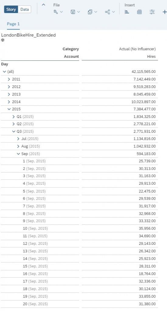
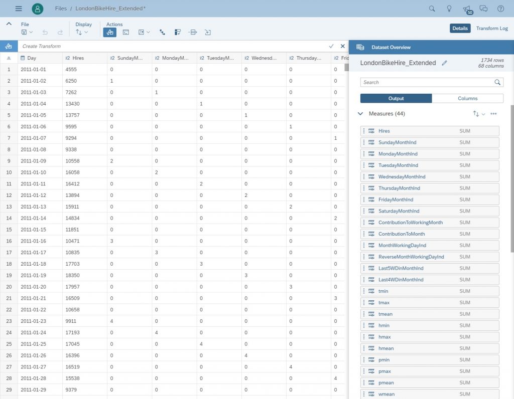
I illustrate my explanations using a bike rental example. The goal is to plan daily hires of bicycle rental in London. To do this I have historical data from 2011 to 20th September 2015. The table below shows for each day the number of bikes hired.
Then I run SAP Predictive Planning from the planning model LondonBikeHire_Extended to get ten predictive forecasts from September 11th to September 20th 2015. So, I can compare actual values of the number of bikes hired with the predictive forecasts.
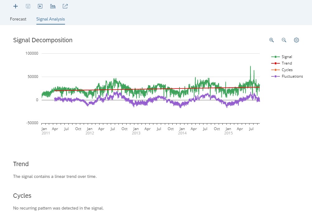
The predictive model I get has a HW-MAPE of 19.74%. In the figure below, only a linear trend and fluctuations are detected. However, there are no recurring cycles detected.
This predictive model gives the forecasts shown below.
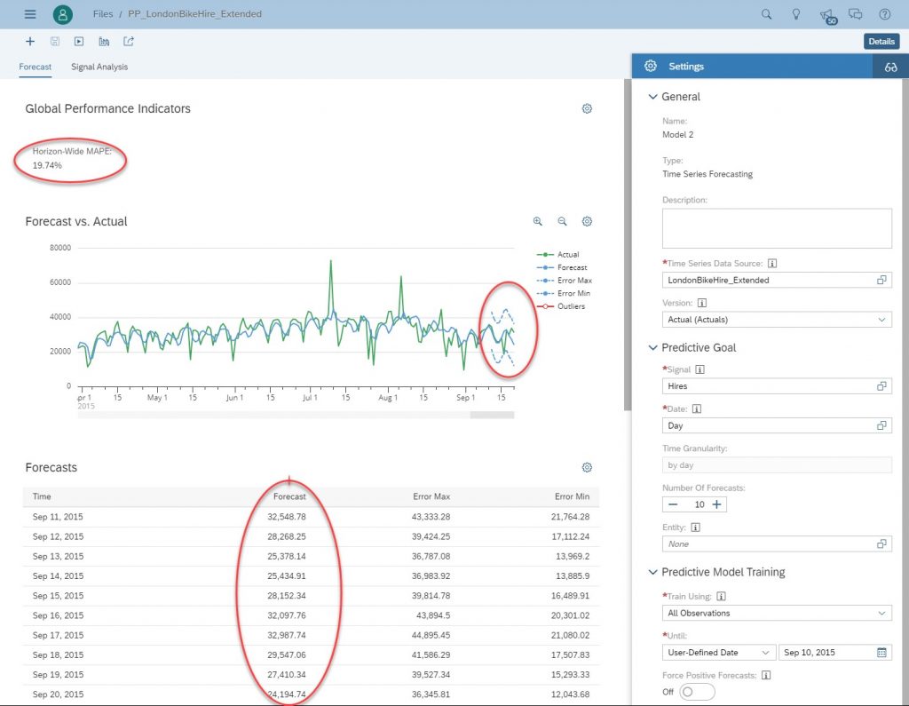
The difference between the Error Max and the Error Min is the confidence interval. On average it is 23,314. It indicates how precise the predictive forecasts are. Now I save these predictive forecasts in a private version of the planning model.
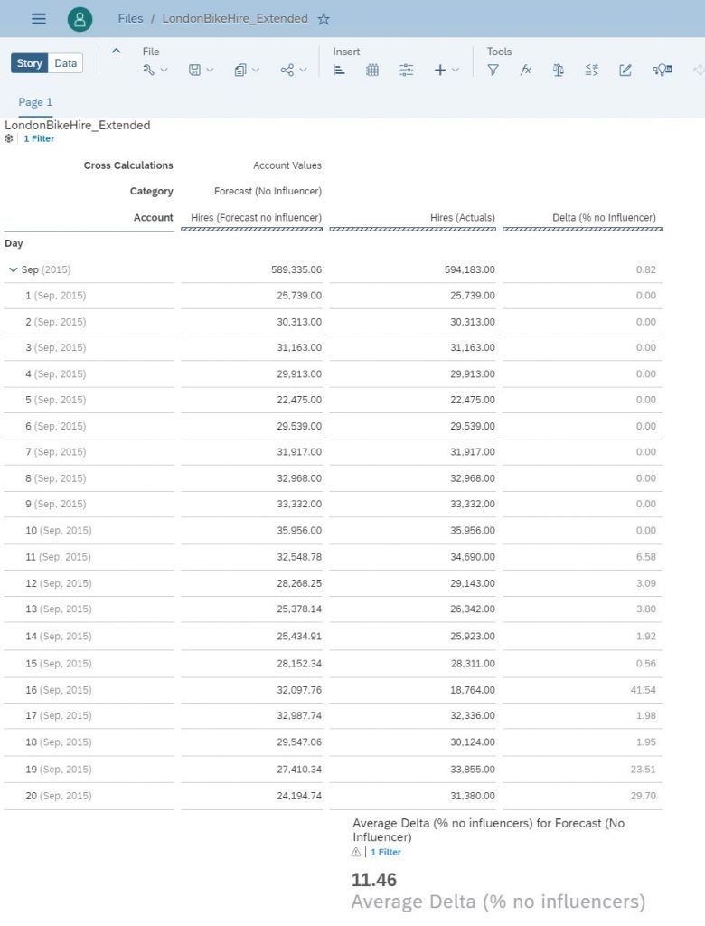
I display actuals & forecasts side by side in a table. I filter on the predicted dates to focus on the comparison between the predictive forecasts for September and the actual values of the hire of bikes. The difference between these values between September 11th and September 20th is on average 11.46%.
Even if these predictive forecasts are accurate, I am not completely satisfied with them, because I feel that I have not used all the information I have. Since the beginning, I have recorded other information like:
- Calendar information (index of the day in the month, is it a working day or a weekend, is it a day off …)
- Weather information (temperature, pressure, is there sun, rain, or cloud …)
- Event information (is it a day during Olympic games or during special event like football or rugby …)
In total, there are 66 other measures and dimensions, and I wonder if they have an influence on my bike hire activity. I want to try out whether including these influencers will improve my predictive forecasts. These measures and the number of bikes hired are recorded into a dataset.
I create a predictive scenario in SAP Smart Predict based on the dataset of figure 5. Then I check if the predictive forecasts are more accurate and I also discover which of my additional variables have the greatest influence. I then save my predictive forecasts into a new dataset, and I link this dataset to my planning story to display the predictive forecasts of my bikes hired. So, let’s do this now.
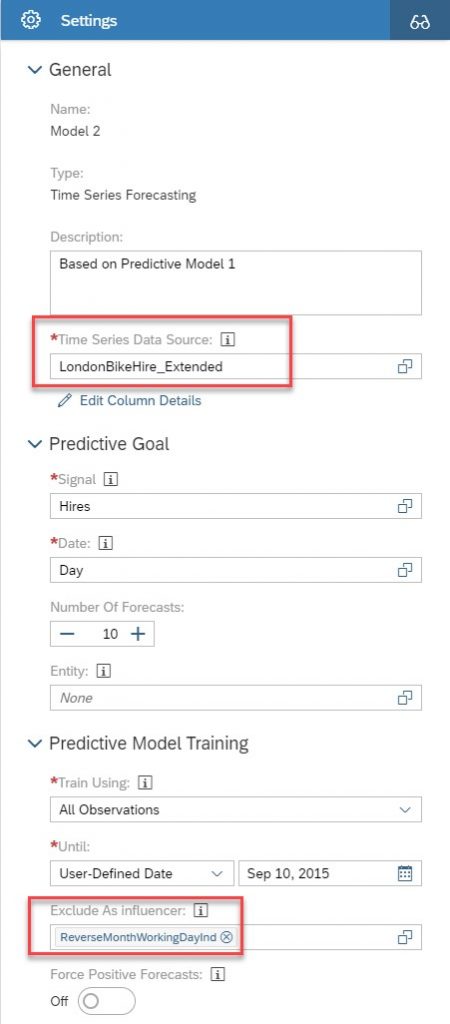
The settings of this predictive scenario are almost the same as those of SAP Predictive Planning. The differences:
- The data source which is now a dataset and
- The field “Exclude As Influencer” set to exclude a variable correlated to the date which does not bring information. I keep all other variables.
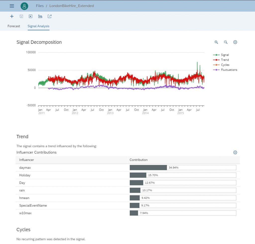
Once trained, the accuracy of the predictive model (HW-MAPE) has a value of 10.66%, which is better than the 19.74% obtained before. The accuracy of the predictive forecasts has increased by 46%.
This time, there are two changes as shown below. The trend is more precise, and is influenced by some of these additional variables. I discover that the trend is influenced at 34.94% by the maximum temperature during the day (daymax). The trend is also influenced at 15.70% if a bike is hired during a weekend, or during a bank holiday. The same way, the bike hire is influenced at 10.17% if it rains.
This predictive model gives the forecasts shown below.
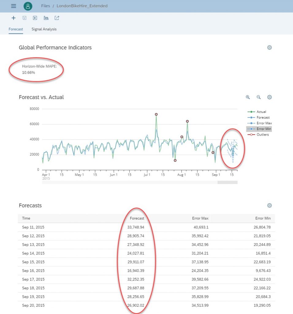
The confidence interval is on average equals to 14,567. It is 37.5% less than in the first predictive model. This also confirm the added value of using influencers.
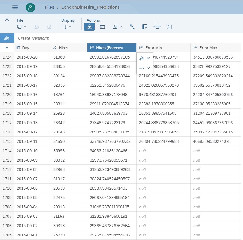
Now I save my predictive forecasts into a dataset named LondonBikeHire_Predictions.
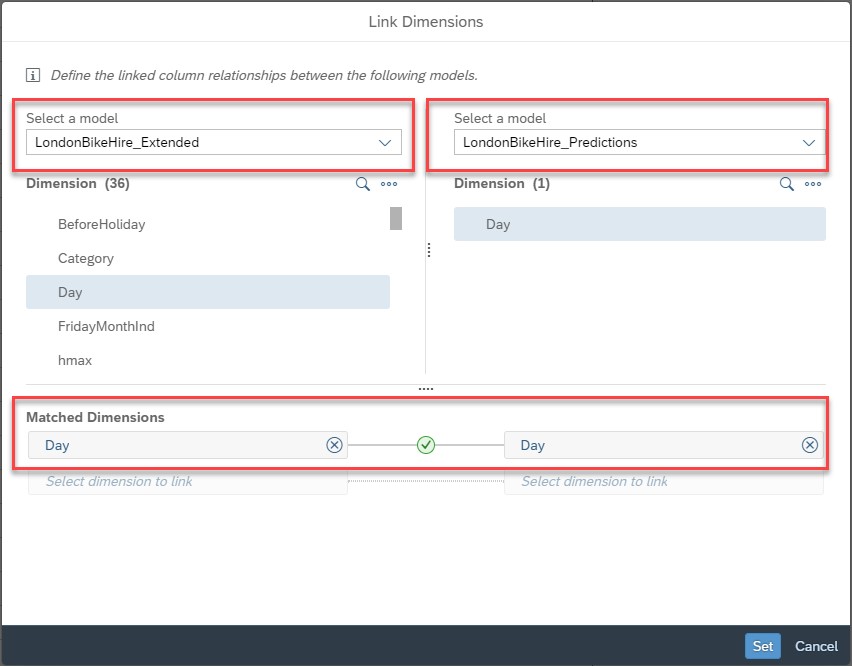
The last step consists of linking this dataset with the planning model in the planning story. For this I just add a linked model with the dataset LondonBikeHire_Predictions and link it on the time dimension to the planning model LondonBikeHire_Extended, as show below.
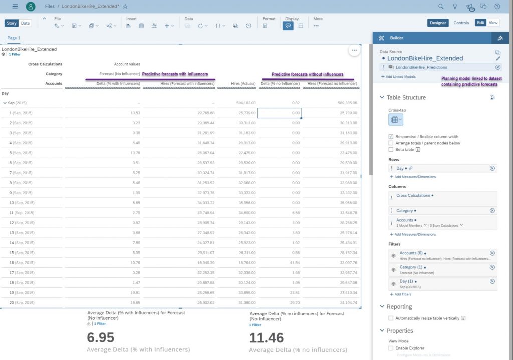
To focus the attention of the predictive forecasts and their comparison with actuals, I filter the time dimension on September 2015. The comparison is done with these calculated measures:
- Delta (% no influencer) is the difference in percentage between predictive forecasts done via SAP Predictive Planning and actual values of the number of bikes hired. The average of this measure is 11.46%.
- Delta (% with Influencers) is the difference in percentage between predictive forecasts done when context is used in the predictive model and actual values of the number of bikes hired. The average of this measure is 6.95%.
What can we conclude? In this case, there are additional variables which have had a positive impact on the accuracy of the predictive model. The Horizon-Wide MAPE is much better (+46%) as well as the confidence interval (+37.5%). This can also be directly confirmed by the smaller gap between predictive forecasts and actual values (39.3% smaller). It is in the interest of the planner to keep in his planning story, the predictive forecasts from the predictive model that were calculated with influencers.
So, in certain cases, adding influencers might help refine the accuracy of the predictive forecast. If this happens with your use cases, you now have a way to bring this added value to your planning stories.


