There are plenty of tutorials on OData but not many are available on XSOData. So we thought of starting a series on this topic which would not only help our readers, but also fine tune our knowledge on these topic.
In this article, we would talk about the SAP Hana Information Modeler and then we would create a Calculation View to understand the different use cases of XSOData.
WHY XSODATA?
We know about OData but WHY we do we need XS?
‘XS’ came from SAP HANA eXtended Application Services which embed a full featured application server, web server, and development environment within the SAP HANA appliance itself. SAP is keen to make our life easy and easy.
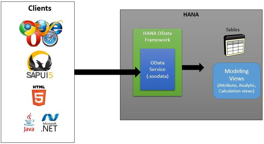
In SAP HANA Extended Application Services(XS), there are different Information Models like Attribute View, Analytical View, Calculation View, Store Procedures and Tables. These can be exposed to clients via a consumption model called XS OData Service and we use OData to enable clients to access data stored in SAP HANA database.
OData Service in SAP HANA XS is defined in a text file with the suffix “.xsodata“. For example “.xsodata”.
Types of Information Models
Three types of Information Views comes under HANA Information modeler:
- Attribute Views
- Analytic Views
- Calculation views
The above views are created from data stored in physical tables of HANA database for analysis using business logic. Meaningful report are created for analysis and research which helps in decision making using these views which are called HANA Database Views(HDB).
Having said that, we may get a question that we have CDS views to create reports , performing complex calculations and stuff like that then why we need these views?
WHY ! WHY ! WHY ! HANA DATABASE VIEWS?
Also, we don’t need anything new until and unless it makes our life simple and these views exactly do that!!
The first and most important point that I think is they provide us option to create views in a graphical interface or in a script editor.With these we can combine data from SAP S/4 any other database tables. It is used to generate complex reports with many calculation option. We have here a data provisioning agent which is used to have other systems in SAP HANA so that we can directly access them in a single platform.
One reason why Information Models were needed is, CDS View were not that powerful during it inceptions. HANA Information Models were the only option then. With S/4HANA and ABAP7.5 CDS Views are on steroids. They have much more capabilities than their predecessors. So in future there might not be anything which CDS would not be able to handle.
Having said that, we would talk about HANA Information Models in this article and prepare another video tutorial on the power and usage of CDS View.
After creating views we can use XSOData service which exposes data stored in views for analysis and executed by front end app. Also, XSOData can be consumed within SAP too and we can have all the data fetched and can utilize them in SAP as per our requirement.
Hands-On Exercise Time
Enough of theory now!! Let’s get to the actual creation of views and XSOdata service. Today, we will focus on Calculation Views (in latest release SAP has marked Attribute and Analytical view as obsolete). Below development is done on HANA WebIDE( it can be done on eclipse also).
As soon as you will open HANA WebIDE, you will get the below screen –
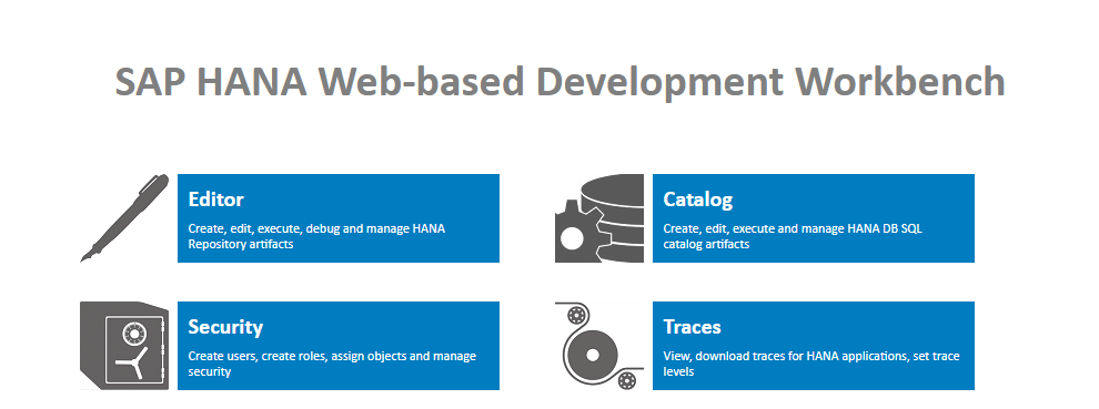
A developer mainly works on first two options, let’s see both one by one .
CATALOG – It contains all available schemas i.e. all data structures, tables and data, column views, procedures that can be used in the content tab.
When we open Catalog we will get below options-
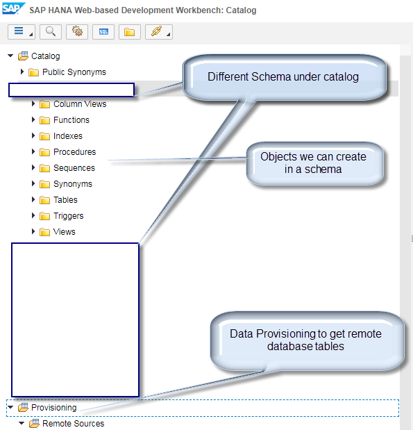
You can play around with all these options and can create a custom schema and tables also and can use the same while creating views.
Now comes the main part of this article:
EDITOR – Holds all information of data models created with the HANA Modeler. These models are organized in Packages. The content node provides different views on the same physical data.
As soon as we open the Editor option we will see the below information:
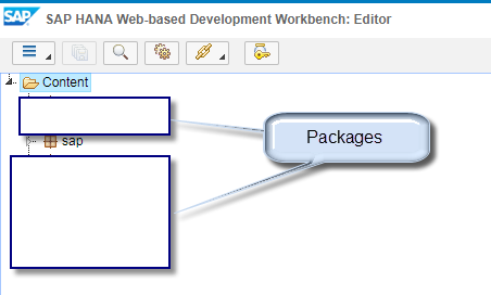
PACKAGES –
Shown under Content tab in HANA. All HANA modeling is saved inside Packages.
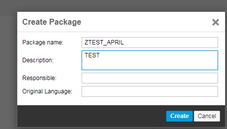
Steps to create Package:
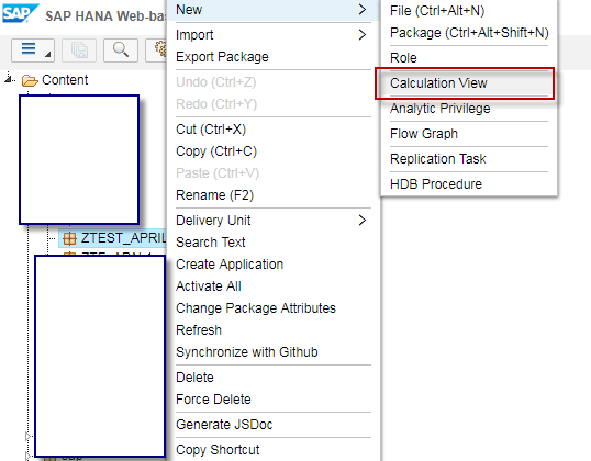
Right Click on Content Tab-> New-> Package. We can create Attribute Views, Analytical Views, and Calculation Views under a Package. Generally, basis team creates a separate package to make any test views so we are going to use the same here.
Below package is created for this article –
Steps to create Calculation View
Now we will create our calculation view under this package as below-
Creation –
– Calculation views are created on the top of tables available in Catalog tab under Schema in HANA and all views are saved under Content tab under a Package –
– It is created to perform complex calculations, which are not possible with other views- Attribute and Analytic views of SAP HANA modeler
– Calculation Views are defined either graphical using HANA Modeling feature or script in the SQL.
– New Views can be created using the two methods given below-
- Graphical
- Script
For our demonstration we will use Graphical Method
We are using graphical method for simplicity and ease of understanding:
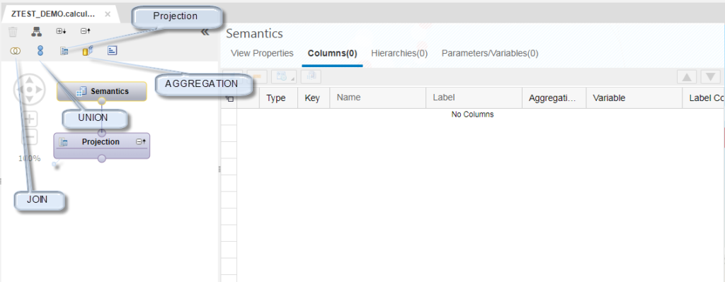
– It has default nodes like Aggregation, Projection, Join and Union.
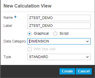
– It can be created using two data category –
i) Cube – Aggregation is default node, one measure is mandatory.
ii) Dimension – Projection is default node
Actual Steps:
1. Right Click Package -> select Calculation View
2. Fill the required fields and click create. I have chosen Dimension data category here for simplicity. We can create cube also and for that one measure is mandatory.
Dimensions:
– Materials, Partners, Employee, Products are Dimensions
– Company’s Master Data are Dimensions
– MARA, LFA1, KNA1, T001 etc are Dimension Tables
KPI (Key Performance Indicator)
– KPIs are numbers (values)
– KPIs are facts
– KPIs are measurable
– Example – Salary, Bonus, Items Sold, Materials Purchased etc
– Since KPIs are numbers and measurable, they are often called Measure
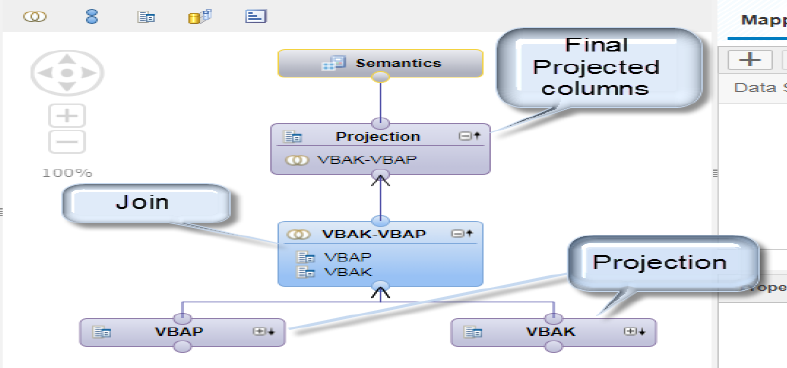
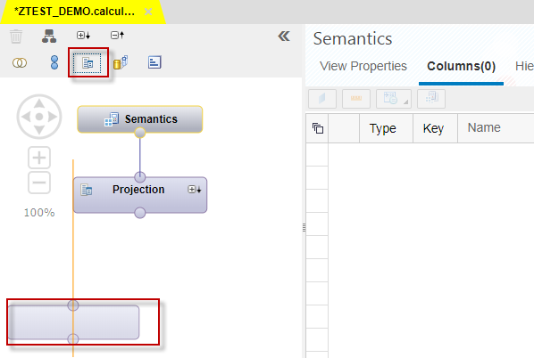
3. Semantics will open for the view where we can create join, union, aggregation etc for the view with the help of database table residing in Catalog tab in HANA Web IDE.
4. We will be creating simple join from two projection of basic tables for practice.
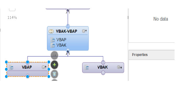
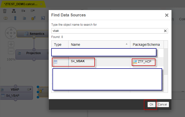
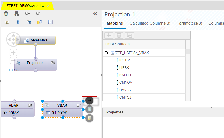
5. To add data source (source table) select Projection and click on ‘+’ symbol and select suitable data source
6. Select VBAK and click ‘OK’
7. Complete the Mapping and drag and drop required columns from data source to output columns, hereafter only output columns will be available for further operations.
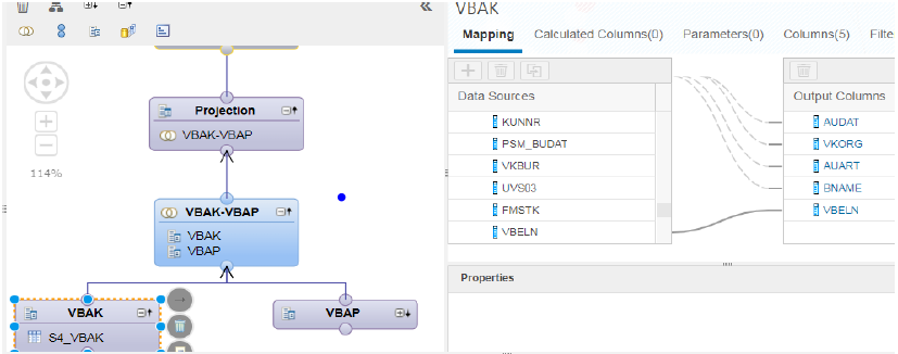
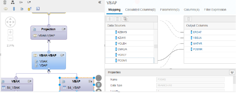
8. Repeat the same steps for VBAP table.
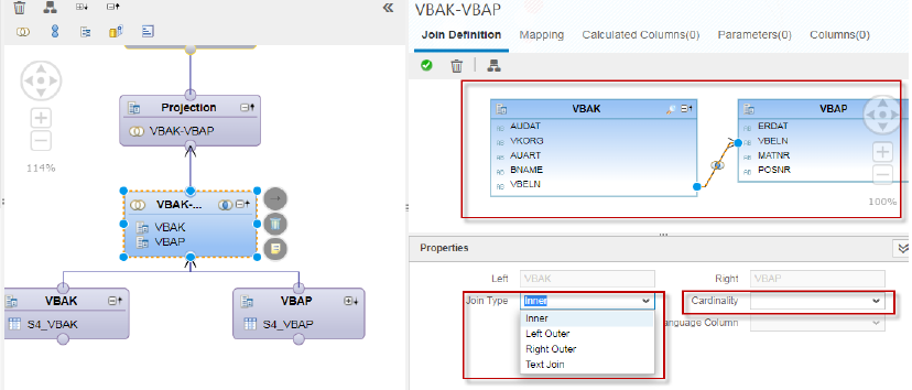
9. Select the Join and Define the join condition, type, cardinality as shown below –
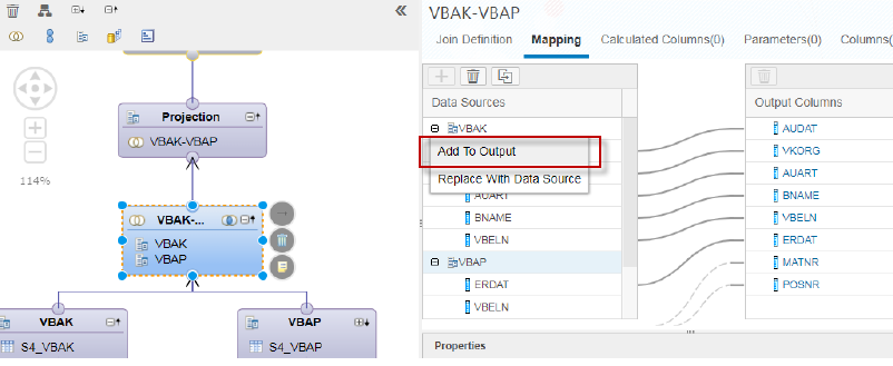
10. Define the mapping and select columns that you want to take forward. You can right click on data source and select add to output to put all columns to output.
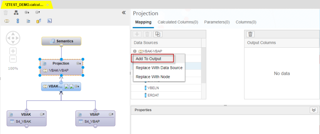
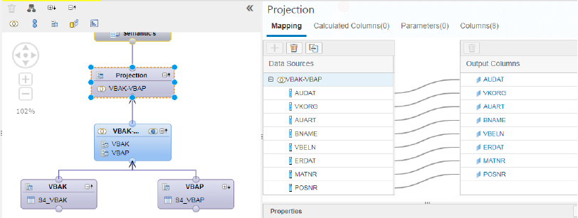
11. Now in Projection tab, define the mapping and select columns for final display.
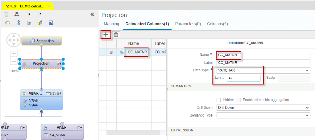
12. Please note, there are Calculated Columns, Parameters tab too. So let’s create a calculated column which will be used heavily in complex reports. I have created a calculated column to add two trailing zeroes in material number. There are many option in elements, functions as shown below which you can explore for different uses.
Click ‘+’ -> provide the required details
Click on Expression Editor to add the expression –
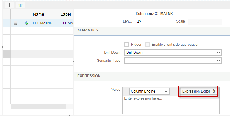
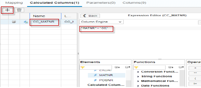
We can either use Column Engine or SQL – both will have different function so we can choose as per our comfort and then can check the syntax using Validate syntax button

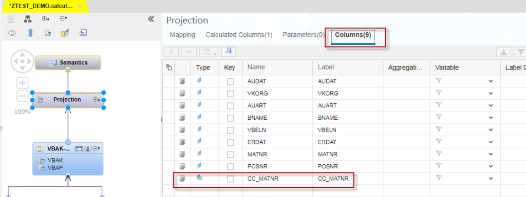
Automatically it will be shown as a new column in the total columns-
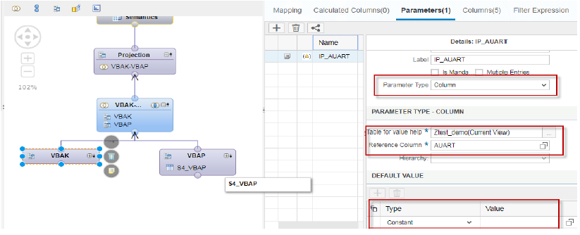
13. Parameter – It can be created at the bottom and can be drilled up to the final output. Creating parameter at bottom (database layer) is useful because it will filter the output at the bottom (db layer) itself to increase the performance.
Parameter Type as Column or Direct, suitable Reference Column and Type as Constant or Expression. For simplicity I am not writing any constant or expression as we are planning to filter output from the service call itself using filter expression.
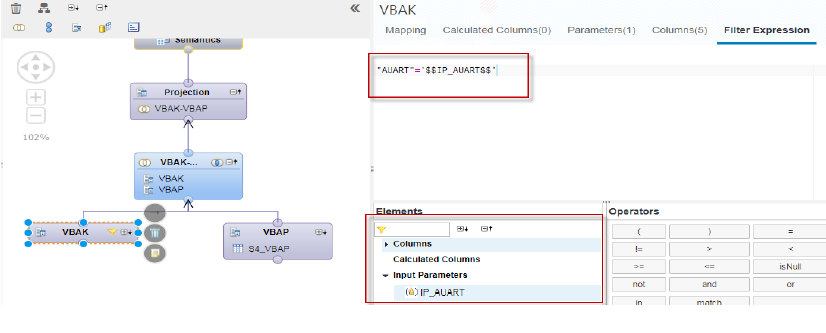
14. Filter Expression – Select suitable columns and input parameter from Elements tab using suitable operator.
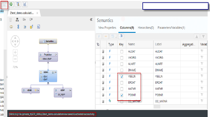
15. Click Semantics where you will see all columns and parameters.
After creating and defining suitable KEYS click save and you will get success or error message in the bottom console window.
16. Now as our calculation view is ready so we need to create XSOData Service to expose the created view by giving the path of the package and view and creating an entity name for our view.
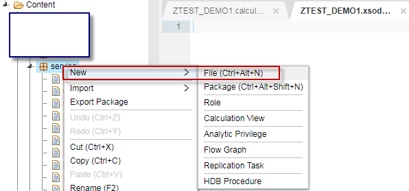
17. Create a new Package as service to keep all the XSOData service separate.
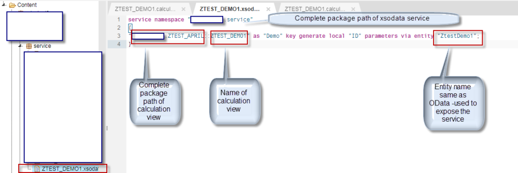
18. Service ZTEST_DEMO1.xsodata is available in package service.
Note – I have renamed the calculation view to ZTEST_DEMO1 as the ZTEST_DEMO has to be used by someone else. Please do not get confused.
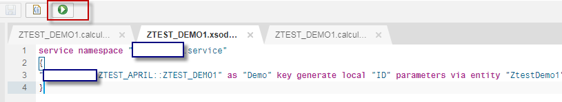
This is the actual step to create XSOData in HANA. Write the service with parameter as shown below:
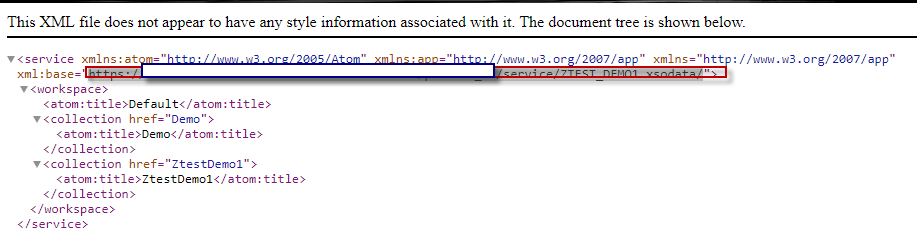
19. Save the service and run it and you will get below output. Copy the highlighted link. Our XSOData entity is created as ZtestDemo1.
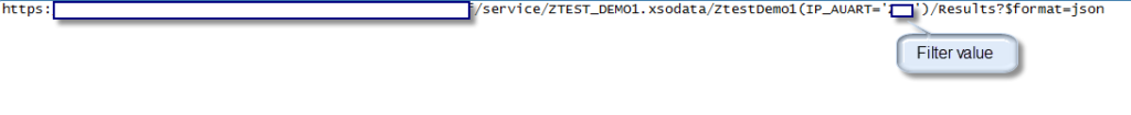
20 Copy the highlighted text and add the entity name with parameter and format details as below. In this case, data is shown as JSON format.
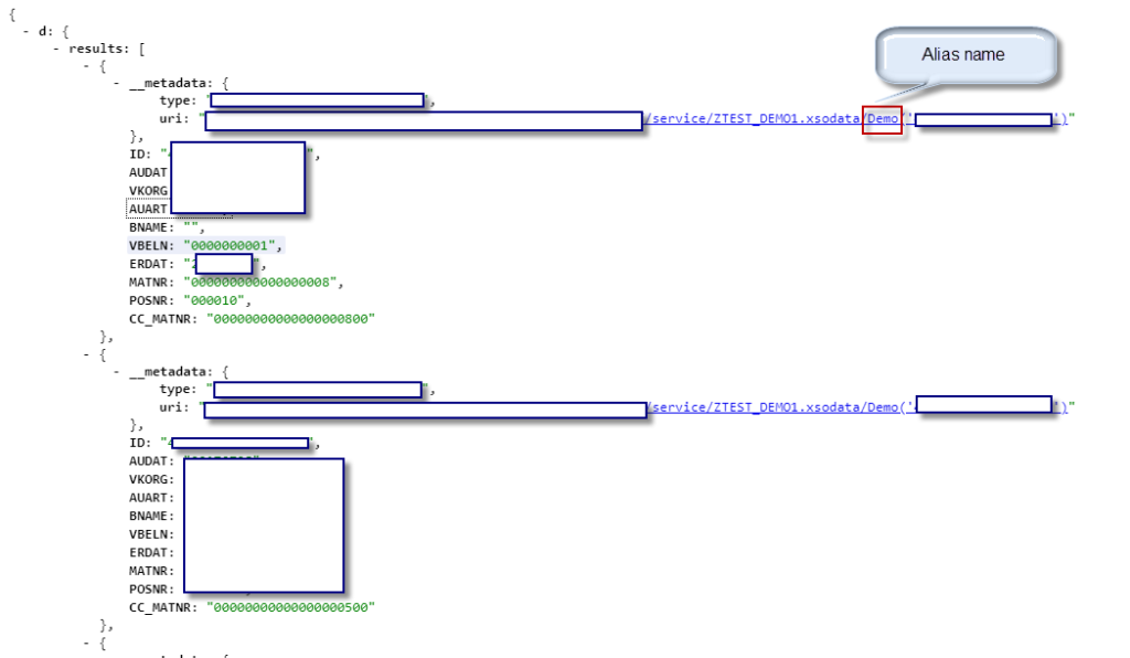
Once you have the XSOData Service created, it behaves like the normal OData Service. We can play around with the Service URI with different query options. Hope you learned something new in this article and we can refer this article in future if we start working on XSOData.


