Find out how to create and deploy SAP HANA Machine Learning pipelines in SAP Data Intelligence. By estimating the price of a used vehicle, we will see how a Data Scientist can work with Python in their familiar Jupyter notebooks with a high degree of agility and how the logic can be deployed into an operational process under the governance of IT.
Begin with exploring and preparing SAP HANA data before deciding on a Machine Learning model. Then move from the creation phase into deployment by leveraging graphical HANA ML operators and templates. You go from raw data to real-time predictions, all without having to extract any data from SAP HANA.
Should you have access to a SAP Data Intelligence system, you can implement this project in your own system. Or you can just read through the article, to get an overview.
Scenario
In this exercise we will estimate the price of a used vehicle. We will train a regression model on the “Ebay Used Car Sales Data“, which contains vehicles that were offered for sale at the end of 2016. The true prices, for which the cars were sold, are not known.
Therefore, to be more precise: we will estimate the price in Euros for vehicles that were offered for sale at the end of 2016. Today’s prices should be lower, with just a few exceptions. Oldtimers tend to get more valuable over time.
System Preparation
For implementing this scenario, you require:
- Access to SAP Data Intelligence
- A SAP HANA system to which SAP Data Intelligence can connect
- A user for that SAP HANA system, which has the rights to call the Predictive Algorithm Library (PAL)
With the above components in place, upload the historic car sales data to SAP HANA. There are many ways for uploading a CSV-file. My favourite option is to load the data from Python directly to SAP HANA. To follow this blog, please use the same approach as this ensures that your data types are in sync with this description.
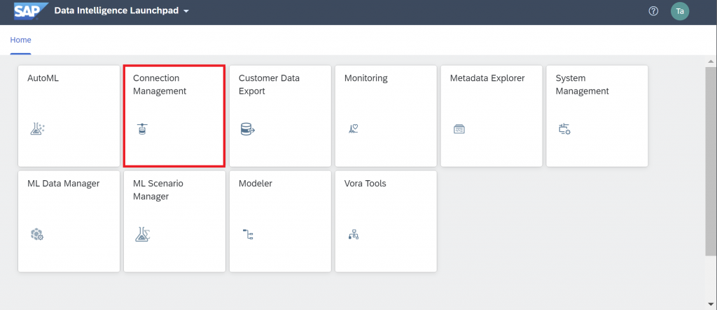
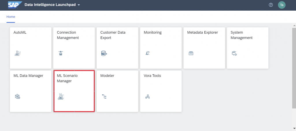
Logon to SAP Data Intelligence and create a connection, which will be used by the notebooks for creating content and by the pipelines for deployment. Select the “Connection Management” tile.
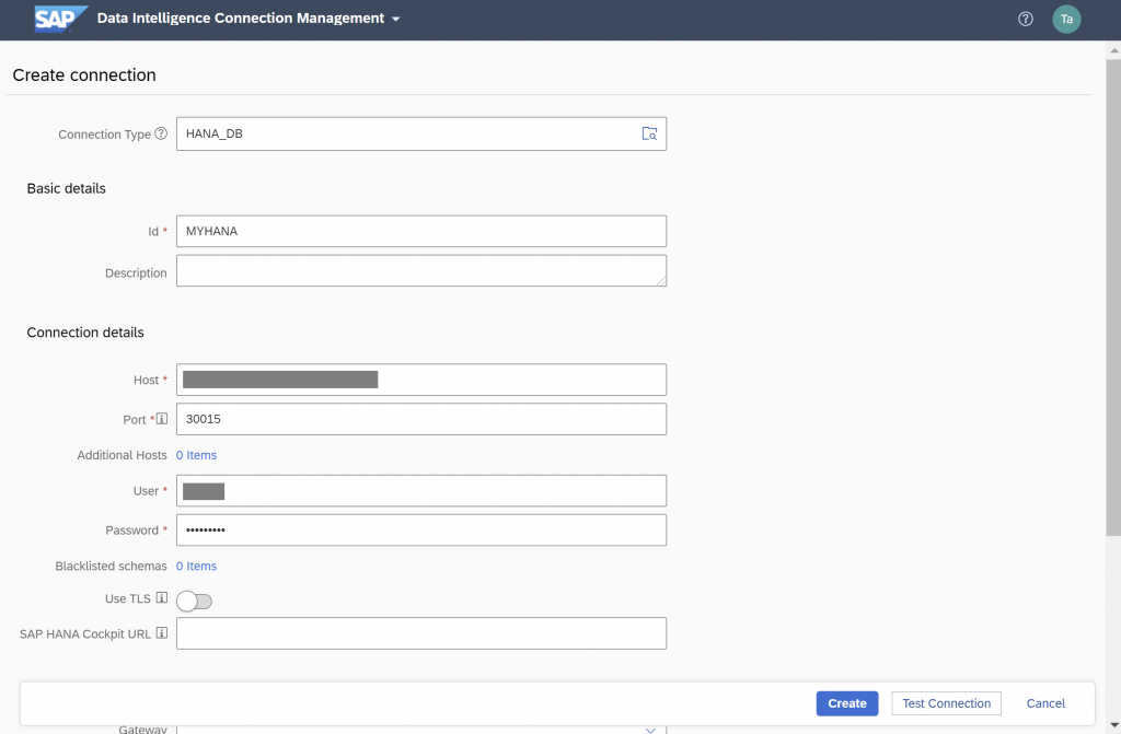
Create a new connection of connection type “HANA_DB”. Name the connection by setting it’s Id to “MYHANA”. Enter the details for your connection.
Back on the Launchpad, click into the “ML Scenario Manager”, from where we will now upload the historic data into SAP HANA. Later on, we will use the same ML Scenario to implement the car price prediction.
In your own, future projects, you may not need to upload any data into SAP HANA. You might be able to work data that is already stored in your existing system.
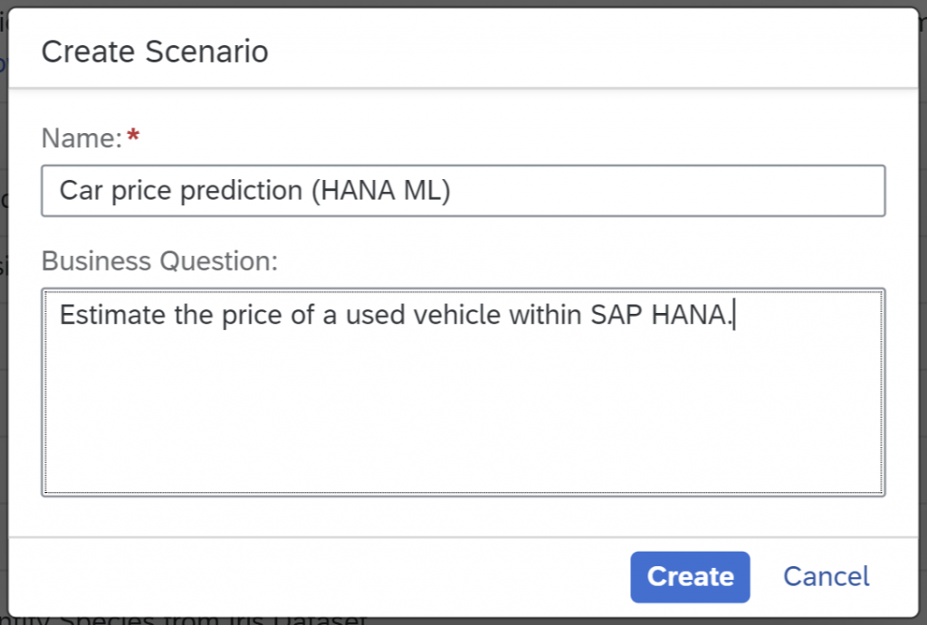
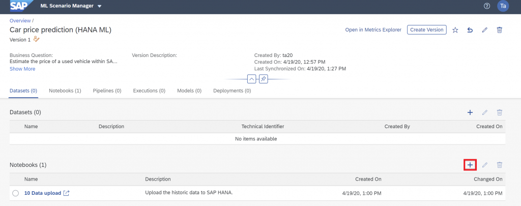
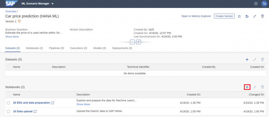
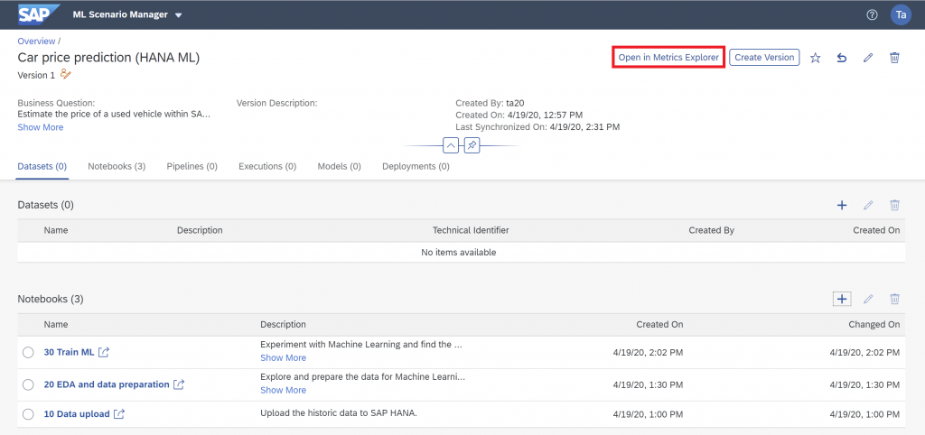
Create a new ML Scenario named “Car price prediction (HANA ML)”.
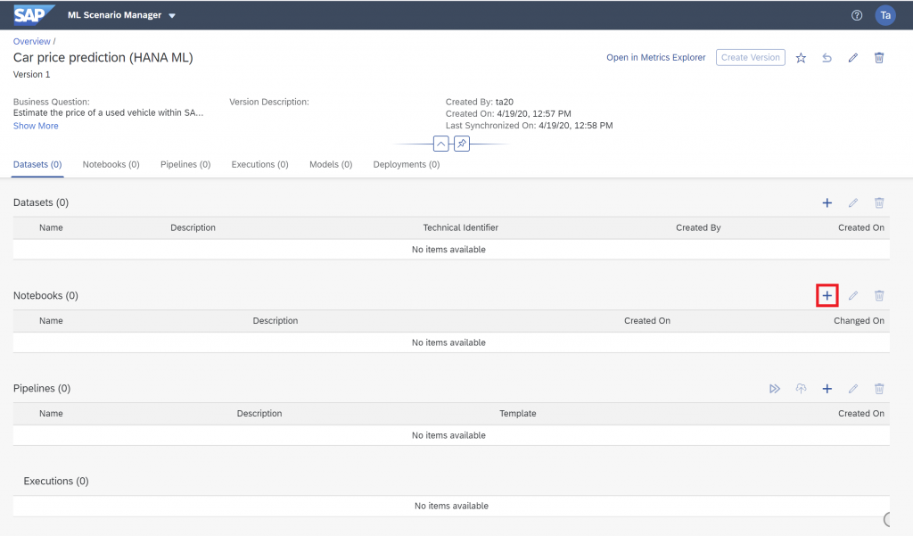
The ML Scenario opens up. Create an empty notebook with the “+”-sign in the Notebooks section.
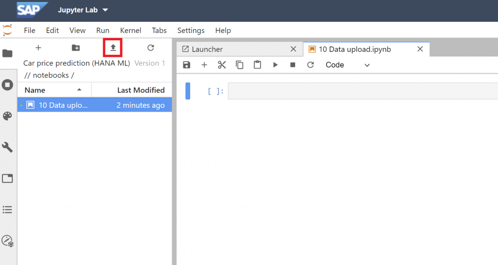
Name the notebook “10 Data upload”. The Jupyter Notebook environment opens up. When prompted for the version of the kernel, select “Python 3”.
Keep the Jupyter window open. Separately, download the file that contains the historic sales data (autos.csv). Unzip the file and upload it into the Notebook environment using the “Upload Files” icon on the left.
Now we can start scripting. We will be using the hana_ml library to upload the data. Later on, we will use the same library for the Machine Learning tasks. The library’s official name is “SAP HANA Python Client API for Machine Learning Algorithms“. There is also a similar hana_ml library for R.
Currently (April 2020) the Jupyter Notebooks in SAP Data Intelligence have an older version of this Python library installed. Verify this for yourself. Enter this Python code in the cell on the right-hand side and execute that cell.
import hana_ml
print(hana_ml.version)
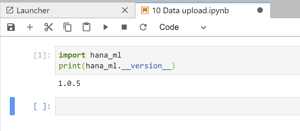
Version 1.0.5 is currently installed. Before continuing, upgrade the library to the latest version.
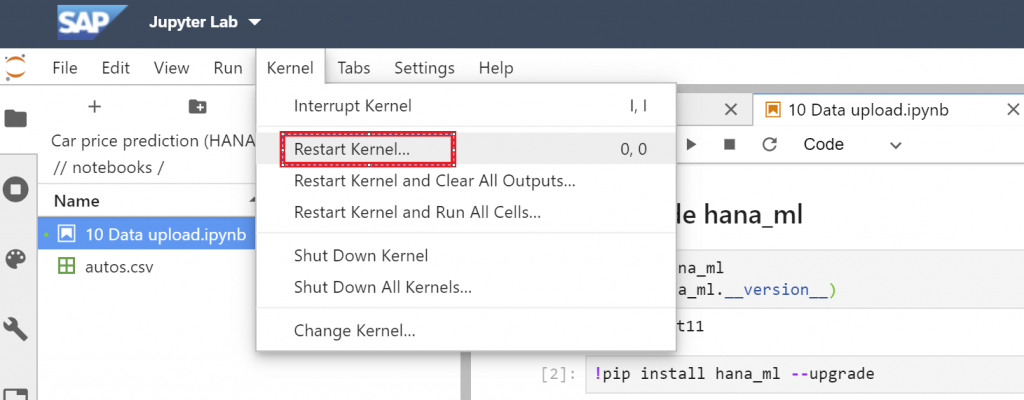
!pip install hana_ml --upgradeRestart the Python kernel, so that your Python session uses the newly installed version.
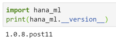
After the restart, verify that the hana_ml library has been upgraded.
import hana_ml
print(hana_ml.__version__)
The library should be at least on version 1.0.8.post11.
Now load the data from the autos.csv file into a Pandas dataframe. Once loaded, it will display the first 5 rows of the data set.
import pandas as pd
df_data = pd.read_csv('autos.csv', encoding = 'Windows-1252')
df_data.head(5)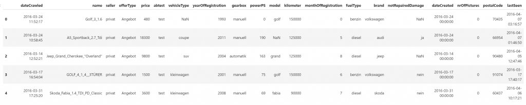
Continue by adjusting the data slightly before uploading it. Turn the column names into upper case.
df_data.columns = map(str.upper, df_data.columns)
Filter the data on Mercedes Benz cars that are offered for sale by private individuals. I just picked a vendor by chance. This exercise is not affiliated with or endorsed by Mercedes Benz in any way.
df_data = df_data[df_data['BRAND'] == 'mercedes_benz']    # Keep only Mercedes Benz
df_data = df_data[df_data['OFFERTYPE'] == 'Angebot']      # Keep only cars for sale (excluding adverts for purchasing a car)
df_data = df_data[df_data['SELLER'] == 'privat']          # Keep only sales by private people (excluding commercial offers)
df_data = df_data[df_data['NOTREPAIREDDAMAGE'] == 'nein'] # Keep only cars that have no unrepaired damage
Remove a few columns for simplicity.
df_data = df_data.drop(['NOTREPAIREDDAMAGE',
                        'NAME',
                        'DATECRAWLED',
                        'SELLER',
                        'OFFERTYPE',
                        'ABTEST',
                        'BRAND',
                        'DATECREATED',
                        'NROFPICTURES',
                        'POSTALCODE',
                        'LASTSEEN',
                        'MONTHOFREGISTRATION'],
                       axis = 1)
Rename some columns for readability.
df_data = df_data.rename(index = str, columns = {‘YEAROFREGISTRATION’: ‘YEAR’,
‘POWERPS’: ‘HP’})
Translate column content from German into English.
df_data['MODEL'] = df_data['MODEL'].replace({'a_klasse': 'A-Class',
                                             'b_klasse': 'B-Class',
                                             'c_klasse': 'C-Class',
                                             'e_klasse': 'E-Class',
                                             'g_klasse': 'G-Class',
                                             'm_klasse': 'M-Class',
                                             's_klasse': 'S-Class',
                                             'v_klasse': 'V-Class',
                                             'cl': 'CL',
                                             'sl': 'SL',
                                             'gl': 'GL',
                                             'clk': 'CLK',
                                             'slk': 'SLK',
                                             'glk': 'GLK',
                                             'sprinter': 'Sprinter',
                                             'viano': 'Viano',
                                             'vito': 'Vito',
                                             'andere': 'Other'
                                             })
df_data['GEARBOX']  = df_data['GEARBOX'].replace({'manuell': 'manual',
                                                  'automatik': 'automatic'})
df_data['FUELTYPE'] = df_data['FUELTYPE'].replace({'benzin': 'petrol'})
Add an ID column, which will be needed for training a Machine Learning model.
df_data.insert(0, 'CAR_ID', df_data.reset_index().index)And move our target column, the price, towards the end. Some algorithms require the target to be the last column of the data. Moving it early on makes it a little easier later on.
df_data = df_data[pd.Index.append(df_data.columns.drop("PRICE"), pd.Index(['PRICE']))]The data is prepared. Now establish a connection to SAP HANA, using the credentials from the MYHANA connection that was created earlier.
import hana_ml.dataframe as dataframe
from notebook_hana_connector.notebook_hana_connector import NotebookConnectionContext
conn = NotebookConnectionContext(connectionId = 'MYHANA')
Upload the data to a table called USEDCARPRICES.
df_remote = dataframe.create_dataframe_from_pandas(connection_context = conn,
                                                   pandas_df = df_data,
                                                   table_name = 'USEDCARPRICES',
                                                   force = True,
                                                   replace = False)
Verify that the data has indeed been uploaded. You could have a look through your usual SAP HANA frontends. Or you can have a look from within the Jupyter Notebook.
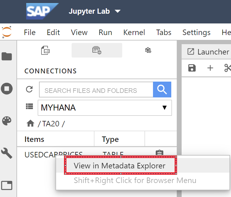
Select the “Data Browser” icon on the very left, then select the “Connections” icon on top and double-click on the “MYHANA” connection.
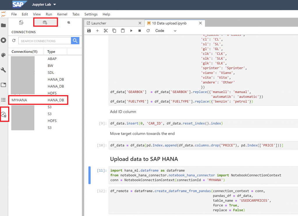
Double-click into your database schema and find the “USEDCARPRICES” table. Now right-click and select “View in Metadata Explorer”.
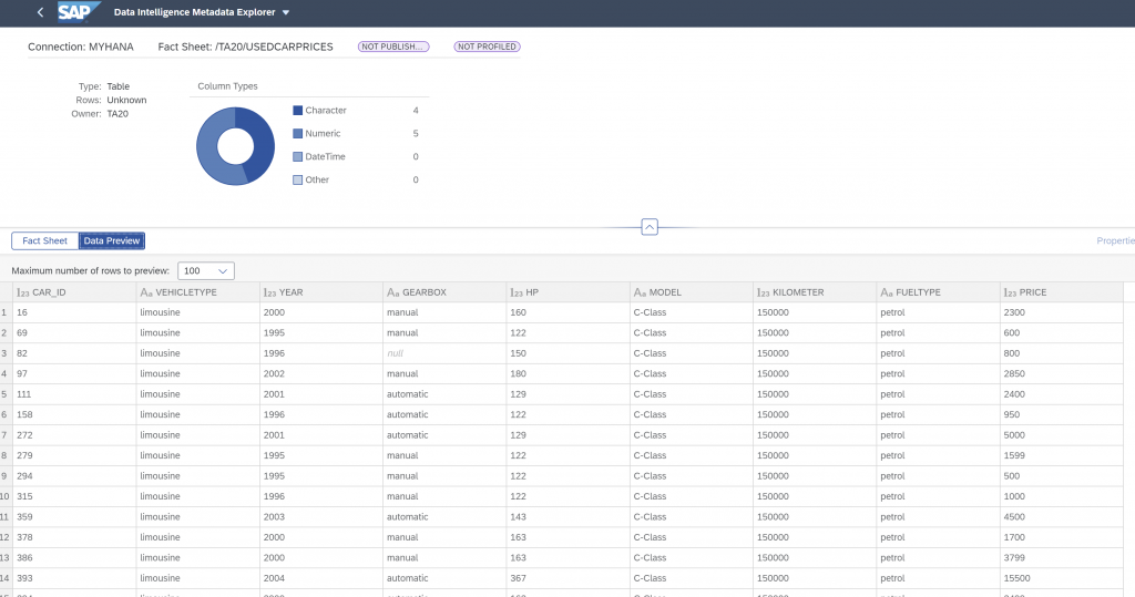
Meta Data Explorer opens up for our new table. Notice that we have 4 columns of type character and 5 numeric columns. Select the *Data Preview” tab and the data should show up!
Back in the notebook close the connection to SAP HANA. Then hit the “Save” icon.
conn.close()Explore and prepare data
The system is ready, the data is loaded. We can start working with the data! On the main page of the ML Scenario create a new notebook called “20 EDA and data preparation”. EDA is a common abbreviation for Exploratory Data Analysis. Once we have explored and understood the data, we prepare it further for Machine Learning.
When the notebook opens, select the “Python 3” kernel as before. Begin by establishing a connection to SAP HANA, leveraging the connection that was centrally defined beforehand.
import hana_ml.dataframe as dataframe
from notebook_hana_connector.notebook_hana_connector import NotebookConnectionContext
conn = NotebookConnectionContext(connectionId = 'MYHANA')
Create a SAP HANA dataframe which points to the USECARPRICES table. Just change the schema name to your own.
df_remote = conn.table(table = 'USEDCARPRICES', schema = '[YOURSCHEMAHERE]')No data gets extracted here from SAP HANA. The object df_remote is a pointer to the table, where the data remains. Try calling the object on its own.
df_remoteNo data is returned, which is good. After all, we want to avoid the movement of data. No data has been extracted yet from SAP HANA. You just see the object type.
However, we can extract data of course if we want to. Python provides an intellisense to see the object’s function. Add a dot after the object name and hit “TAB” on your keyboard.
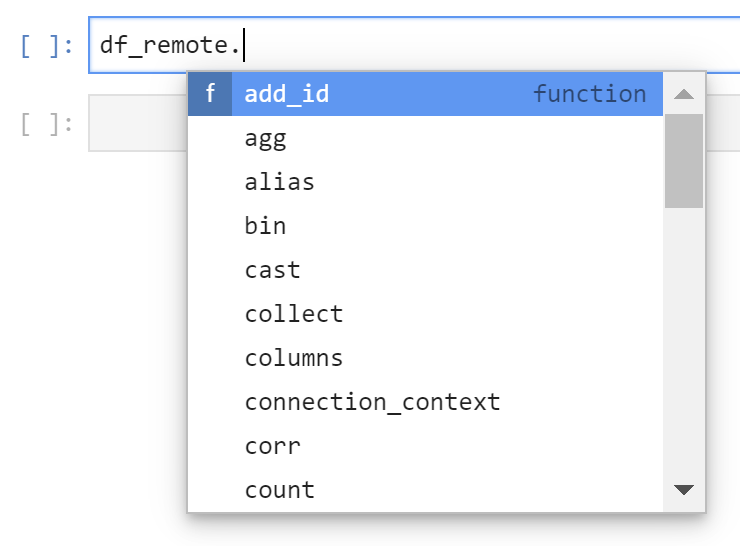
Knowing which functions are available and how to use them will come in handy during any project. Select the head() function to specify a small number of rows. Place the cursor into the function’s round brackets, then hit SHIFT + TAB and the intellisense shows the help for this function, i.e. what it does, and which parameters can be passed into it.
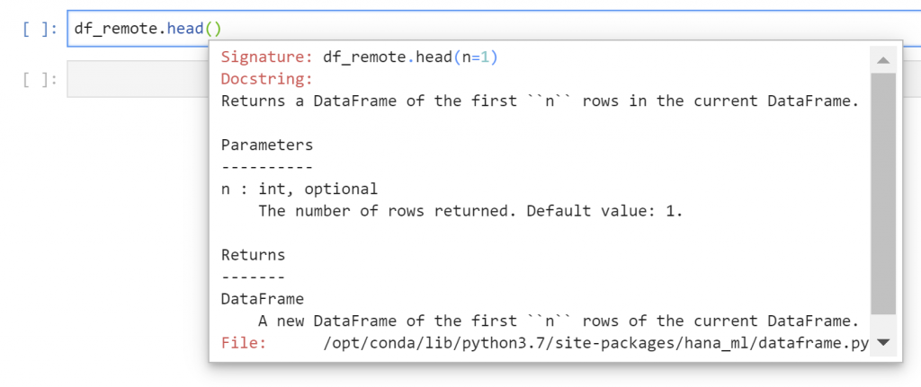
Retrieve 5 rows from the table. The collect function is needed to transfer the data into Python. It is important to restrict the data first (with the head function) before extracting it with the collect function.
df_remote.head(n = 5).collect()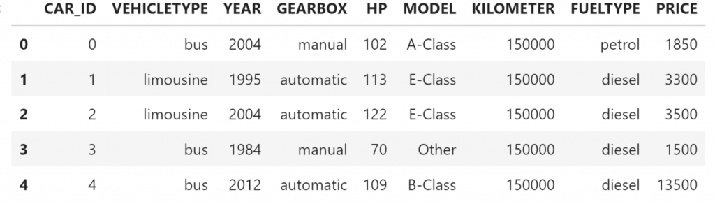
Continue by exploring the data. Count the number of rows for instance.
df_remote.count()Find the price of the most expensive car.
df_remote.agg([('max', 'PRICE', 'MOSTEXPENSIVE')]).collect()Use the describe function, to get an overview of the content of all columns.
df_remote.describe().collect()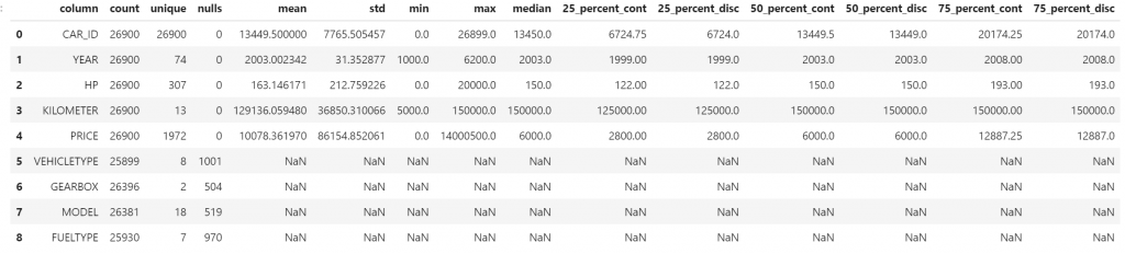
Each cell was calculated by SAP HANA. Only the results were then moved to Python. In that table you will also find the values that you had requested earlier, i.e. the price of the most expensive car.
To prove the point that SAP HANA did the work here, ask for the underlying SELECT statement, which was created by the hana_ml library.
df_remote.describe().select_statementThe SQL syntax that is displayed, is much too long to be displayed here. However, seeing that SQL code might also help understand how the hana_ml library works, how it translates the requests into SQL code for SAP HANA.
Continue the exploration by finding the most frequent car models in the data set.
top_n = 5
df_remote_col_frequency = df_remote.agg([('count', 'MODEL', 'COUNT')],  group_by = 'MODEL')
df_col_frequency = df_remote_col_frequency.sort('COUNT', desc = True).head(top_n).collect()
df_col_frequency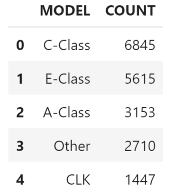
Plot the data of the above Pandas dataframe.
%matplotlib inline
df_col_frequency.plot.bar(x = 'MODEL',
                          y = 'COUNT',
                          title = 'Top ' + str(top_n));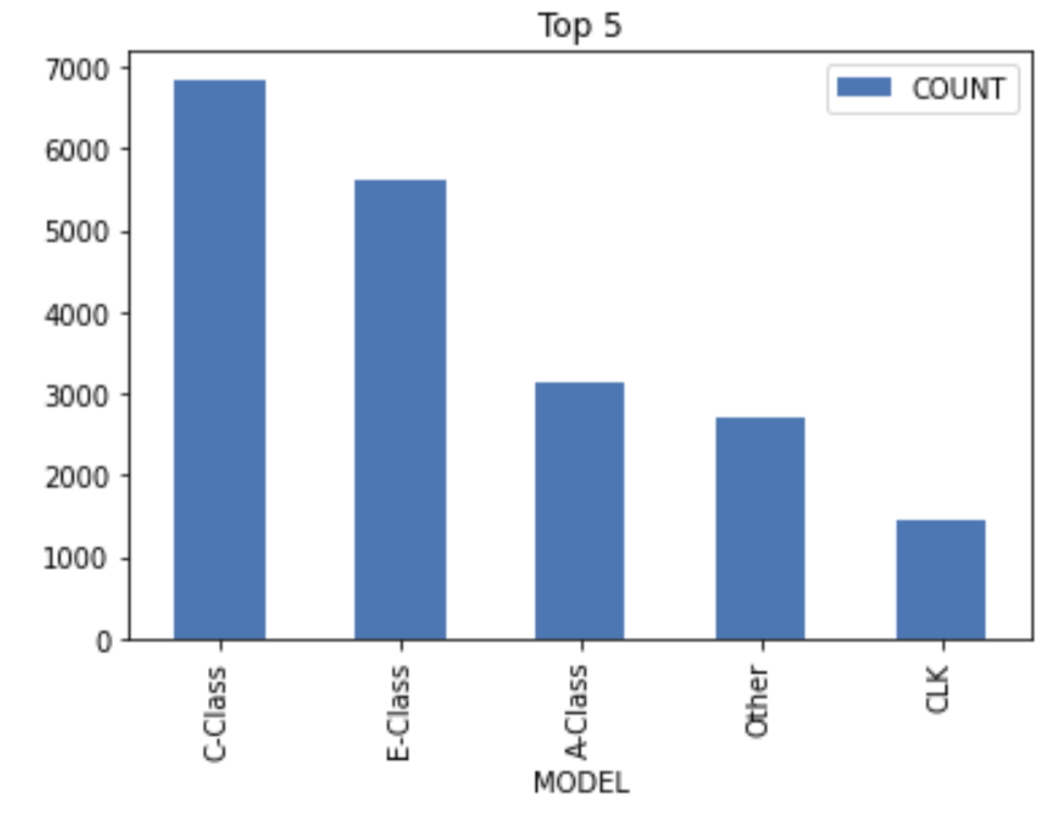
Inspect the price of a car against the year in which it was built. First install the seaborn library for additional charting capabilities.
!pip install seabornFor a small sample of all cars retrieve only the year and the price.
col_name_1 = 'PRICE'
col_name_2 = 'YEAR'

from hana_ml.algorithms.pal import partition
df_remote_sample, df_remote_ignore1, df_remote_ignore2 = partition.train_test_val_split(
                               conn_context = conn,
                               data = df_remote,
                               random_seed = 1972,
                               training_percentage = 0.01,
                               testing_percentage = 0.99,
                               validation_percentage = 0)
df_sample = df_remote_sample.select(col_name_1, col_name_2).collect()
Visualise the data in a scatter plot.
%matplotlib inline
import seaborn as sns
sns.jointplot(x=col_name_1, y=col_name_2, data=df_sample);
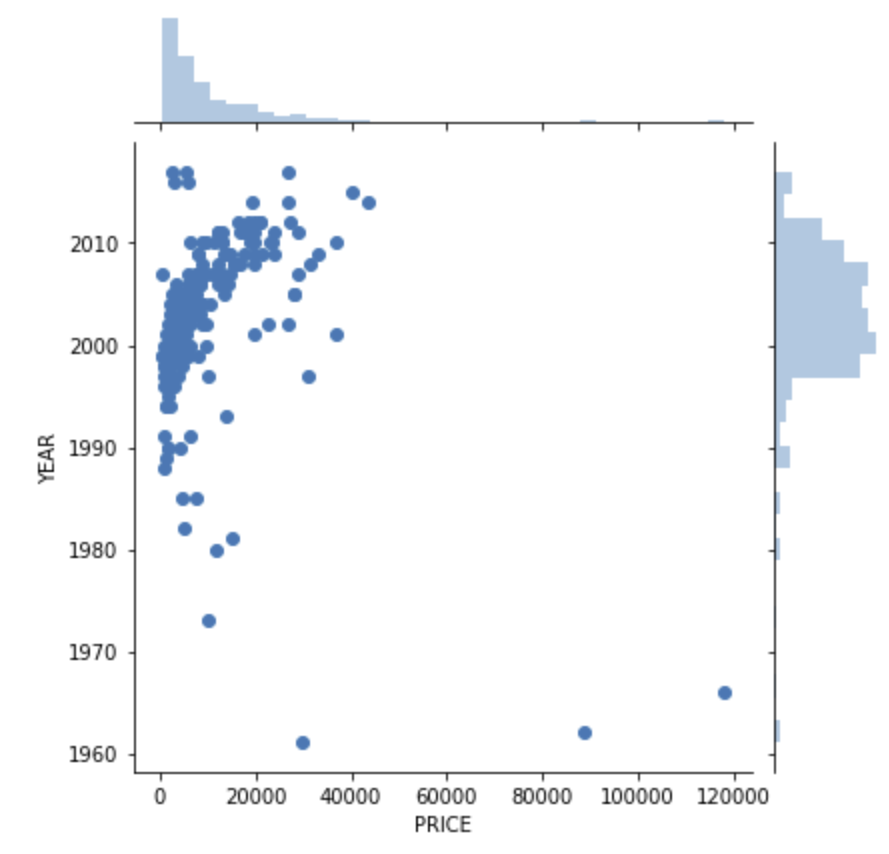
For newer cars there is a trend that they are more expensive. However, the most expensive cars are the oldest ones. That’s the oldtimers. Therefore, filter the dataset to focus on the more common cars. Only consider cars that were built in the year 2000 or later and that cost under 50.000 Euros. And to keep things a little simple for now, all rows with missing values are also dropped. 18066 cars remain.
df_remote = df_remote.filter('YEAR >= 2000')
df_remote = df_remote.filter('PRICE < 50000')
df_remote = df_remote.dropna()
df_remote.count()
Continue by analysing the correlations between the numerical variables.
import matplotlib.pyplot as plt
from hana_ml.visualizers.eda import EDAVisualizer
f = plt.figure()
ax1 = f.add_subplot(111) # 111 refers to 1x1 grid, 1st subplot
eda = EDAVisualizer(ax1)
ax, corr_data = eda.correlation_plot(data = df_remote.drop(['CAR_ID']),
                                     cmap = 'coolwarm')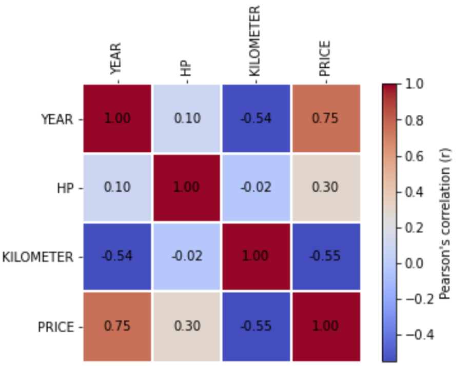
The strongest positive correlation exists between the year in which the car was built and the price with a coefficient of 0.75. That means, there is a fairly strong trend that newer cars come with a higher price. Or vice versa, older cars tend to be cheaper. Similarly, the negative correlation of -0.55 between the price and kilometer means, that a higher mileage tends to come with a lower price. Or the other way round. Both make perfect sense of course.
We have a reasonable understanding of the data now. Before making the prepared data available for Machine Learning, just convert the target column of our prediction, the price, into a DOUBLE type. This will be needed later or by the algorithm that trains the model. Converting it early, makes things a little easier later on.
df_remote = df_remote.cast('PRICE', 'DOUBLE')Now that the data is fully prepared, save it as a view to SAP HANA. This function returns a SAP HANA dataframe, which points to the newly created view. Hence Python will display the object type hana_ml.dataframe.DataFrame. This is not an error; you have already seen this behaviour at the beginning of this notebook.
df_remote.save(where = ('[YOURSCHEMAHERE]', 'USEDCARPRICES_PREPVIEW'), table_type = 'VIEW', force = True)Close the connection and save the notebook.
conn.close()
The original data in the USEDCARPRICES table remains unchanged. No data has been duplicated, but the view USEDCARPRICES_PREPVIEW now provides suitable data for the purpose of Machine Learning.
Train ML model
For the Machine Learning part, I prefer to use a separate notebook. Create a new notebook named “30 Train ML”. Select the “Python 3” kernel when prompted.
Begin by establishing a connection to SAP HANA again.
import hana_ml.dataframe as dataframe
from notebook_hana_connector.notebook_hana_connector import NotebookConnectionContext
conn = NotebookConnectionContext(connectionId = 'MYHANA')
Create a SAP HANA dataframe, that now points to the view that represents the prepared and filtered data.
df_remote = conn.table(table = 'USEDCARPRICES_PREPVIEW', schema = '[YOURSCHEMAHERE]')Peek at the data, retrieve 5 rows.
df_remote.head(5).collect()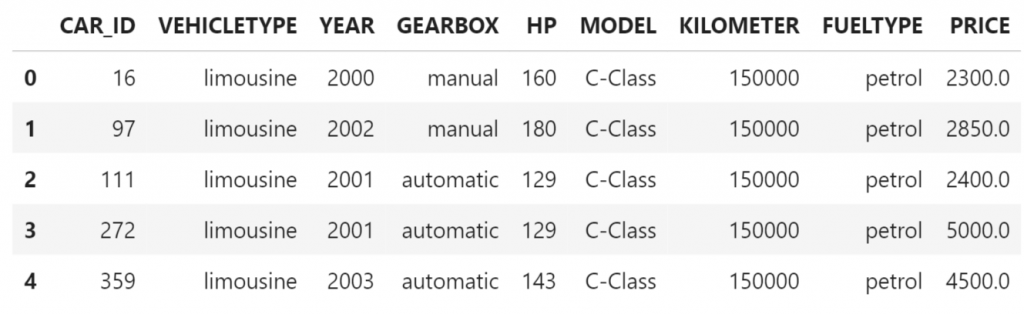
Before training any Machine Learning model, split the data into two separate parts. One part (70%) will be used to train different ML models. The other part (30%) will be used to test the model’s quality.
from hana_ml.algorithms.pal import partition
df_remote_train, df_remote_test, df_remote_ignore = partition.train_test_val_split(conn_context = conn,
                                                                                   random_seed = 1972,
                                                                                   data = df_remote,
                                                                                   training_percentage = 0.7,
                                                                                   testing_percentage = 0.3,
                                                                                   validation_percentage = 0)
See how many rows are in each subset.
print('Size of training subset: ' + str(df_remote_train.count()))
print('Size of test subset: ' + str(df_remote_test.count()))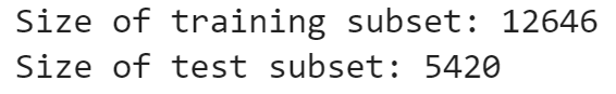
Use the training data to train a very first Hybrid Gradient Boosting regression. The code specifies the regression’s target (PRICE), predictor columns (i.e. YEAR and HP) as well which hyperparameters to use for training the algorithm. For now, we are not too concerned about the model quality. This step is primarily to show the concept how such a model can be trained. Later on we will try to improve the model.
from hana_ml.algorithms.pal import trees
hgb_reg = trees.HybridGradientBoostingRegressor(conn_context=conn,
                                                random_state = 42,
                                                n_estimators = 10,
                                                max_depth = 5,
                                                learning_rate = 0.3,
                                                min_sample_weight_leaf = 1,
                                                min_samples_leaf = 1,
                                                lamb = 1,
                                                alpha = 1)

# Specify the model's predictors
features = ['YEAR', 'HP', 'KILOMETER', 'VEHICLETYPE', 'GEARBOX', 'MODEL', 'FUELTYPE']

# Train the model
hgb_reg.fit(data = df_remote_train,
            features = features,
            key = "CAR_ID",
            label = 'PRICE')
With the trained model, we can test its performance on the test data. First compare the actual / true price of the car from the test data with the prediction of the regression model.
df_remote_act_pred = df_remote_test.alias('L').join(
    hgb_reg.predict(data = df_remote_test, features = features, key = 'CAR_ID').alias('R'),
    'L.CAR_ID = R.CAR_ID',
    select=[('L.CAR_ID', 'CAR_ID'), 'MODEL', ('PRICE','ACTUALS'), ('SCORE', 'PREDICTIONS')])
df_remote_act_pred.head(5).collect()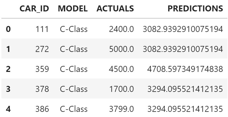
Some predictions are closer to the actual value than others. Now calculate the Root Mean Squared Error (RMSE), which gives an indication of the model’s overall performance for all cars in the test dataset.
import numpy as np
df_remote_se = df_remote_act_pred.select('CAR_ID',
                                        'ACTUALS',
                                        'PREDICTIONS',
                                        ('(ACTUALS - PREDICTIONS) * (ACTUALS - PREDICTIONS) ', 'ERRORSQ'))
df_mse = df_remote_se.agg([('avg', 'ERRORSQ', 'MSE')]).collect()
rmse = np.sqrt(float(df_mse.iloc[0:,0]))
print('RMSE: ' + str(round(rmse, 2)))
The RMSE is about 3096. This means a little simplified, that by this definition, the model was on average 3096 Euros away from the true value. That can be good or bad, depending on the circumstances.
Now however, we want to improve the quality of the model. We stick with the same algorithm, but we try out different hyperparameter values (i.e. for n_estimator or max_depth) to achieve a lower RMSE on the test data.
These hyperparameter values will be tested.
n_estimators = [10, 20, 30, 40, 50]
max_depth = [2, 3, 4, 5, 6, 7, 8, 9, 10]
In this loop, all hyperparameter combinations are tested. A model is trained on the training data, the RMSE is calculated on the test data. The results are stored both in Python as well as in the ML Scenario. Running this cell will take a few minutes…
import pandas as pd
from math import sqrt
from sapdi import tracking

# Dataframe to store hyperparameters with model quality
df_hyper_quality = pd.DataFrame(columns=['N_ESTIMATORS', 'MAX_DEPTH', 'RMSE'])

# Iterate through all parameter combinations
from hana_ml.algorithms.pal import trees
for aa in n_estimators:
    for bb in max_depth:
        hgb_reg = trees.HybridGradientBoostingRegressor(conn_context=conn,
                                                random_state = 42,
                                                min_samples_leaf = 1,
                                                n_estimators = aa,
                                                max_depth = bb)

        # Train the regression with the current parameters
        hgb_reg.fit(data = df_remote_train,
                       features = features,
                       key = "CAR_ID",
                       label = 'PRICE')

        # Evaluate the model on the test data
        df_remote_act_pred = df_remote_test.alias('L').join(
                                hgb_reg.predict(data = df_remote_test, features = features, key = 'CAR_ID').alias('R'),
                                'L.CAR_ID = R.CAR_ID',
                                select=[('L.CAR_ID', 'CAR_ID'), ('PRICE','ACTUALS'), ('"SCORE"', 'PREDICTIONS')])
        df_remote_se = df_remote_act_pred.select('CAR_ID',
                                                     'ACTUALS',
                                                     'PREDICTIONS',
                                                     ('(ACTUALS - PREDICTIONS) * (ACTUALS - PREDICTIONS) ', 'ERRORSQ'))
        df_mse = df_remote_se.agg([('avg', 'ERRORSQ', 'MSE')]).collect()
        rmse = np.sqrt(float(df_mse.iloc[0:,0]))

        # Print a status update
        print('n_estimators: ', aa, ' | max_depth: ', bb)
        print('RMSE on test data: ' + str(round(rmse, 2)))
        print()

        # Add the parameters and the RMSE to the collection in Python
        df_hyper_quality = df_hyper_quality.append({'N_ESTIMATORS': aa,
                                                    'MAX_DEPTH': bb,
                                                    'RMSE': rmse},
                                                    ignore_index = True)

        # Add the parameters and RMSE to the ML Scenario
        run = tracking.start_run(run_collection_name="Car price experiments")
        tracking.log_parameters({"n_estimators": aa,
                                 "max_depth": bb})
        tracking.log_metrics({"RMSE": rmse})
        tracking.end_run()

print('Done')
Once the cell has completed, see which model performed best.
df_hyper_quality.sort_values(by = 'RMSE', ascending = True).head(5)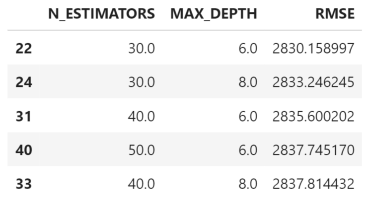
The model that was trained with n_estimators = 30 and max_depth = 6 resulted in the lowest RMSE. We could already deploy this model now in a graphical pipeline, but let’s have a closer look at the model beforehand. Train the model once more, now with those identified hyperparameter values. Please note, that the process has some randomness and that your best hyperparameter values might be different.
hgb_reg = trees.HybridGradientBoostingRegressor(conn_context=conn,
                                                random_state = 42,
                                                n_estimators = 30,
                                                max_depth = 6,
                                                min_samples_leaf = 1)
hgb_reg.fit(data = df_remote_train,
            features = features,
            key = "CAR_ID",
            label = 'PRICE')
Compare the actuals with the predicted values.
df_remote_act_pred = df_remote_test.alias('L').join(
    hgb_reg.predict(data = df_remote_test, features = features, key = 'CAR_ID').alias('R'),
    'L.CAR_ID = R.CAR_ID',
    select=[('L.CAR_ID', 'CAR_ID'), 'MODEL', ('PRICE','ACTUALS'), ('SCORE', 'PREDICTIONS')])
df_remote_act_pred.head(5).collect()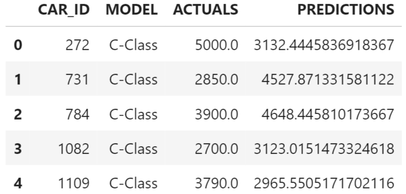
As a test, calculate the RMSE. This should result in the same value as before when this model was identified as the strongest.
import numpy as np
df_remote_se = df_remote_act_pred.select('CAR_ID',
                                             'ACTUALS',
                                             'PREDICTIONS',
                                             'MODEL',
                                             ('(ACTUALS - PREDICTIONS) * (ACTUALS - PREDICTIONS) ', 'ERRORSQ'))
df_mse = df_remote_se.agg([('avg', 'ERRORSQ', 'MSE')]).collect()
rmse = np.sqrt(float(df_mse.iloc[0:,0]))
print('RMSE: ' + str(round(rmse, 2)))
Finally, investigate how well the model performs by car model.
df_mse = df_remote_se.agg([('avg', 'ERRORSQ', 'MSE')], group_by = ['MODEL']).collect()
df_mse['RMSE'] = np.sqrt(df_mse['MSE'])
df_mse.sort_values(by = ['RMSE'], ascending = True)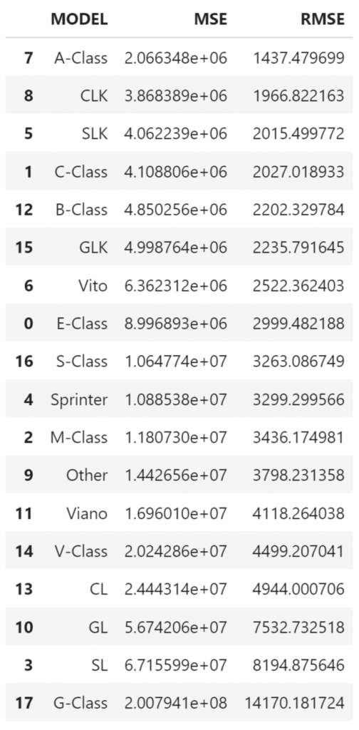
The model performed best on the A-Class. This is not very surprising as this is a lower priced model. Since we measure the quality of the prediction in absolute Euros (and not in percentage for instance), the prediction errors in Euros should not be very high for the A-Class. The G-Class however, for which the model as a much large RMSE, is a more expensive model. One could consider training a separate model for the G-Class, but we will go with the model now as it is.
Close the connection and save the notebook.
conn.close()
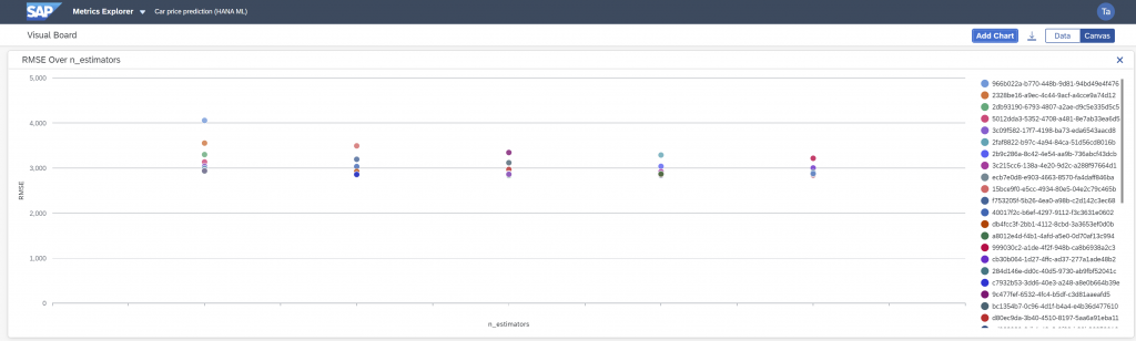
Earlier on, when the different parameter combinations for the model were tried out, for each model the parameters and the resulting RMSE was saved into the ML Scenario (see the “tracking” commands). Those values can be helpful for transparency. In case you need to recall at some point in the future, which models were considered, they are persisted here.
Back in the ML scenario you click “Open in Metrics Explorer”.
You will first see a tabular display of the information, but the data can also be charted. It’s fairly easy to find your way around, just give it a try if you are interested. (In the Metrics Explorer select the collection of metrics on the left → Select all runs → click “Open Visual Board” → “Canvas” → “Add Chart” → “Plot Metric against Parameter”)
Training pipeline
Through the above work in the notebooks we know which algorithm and which hyperparameters we want to use for the ML model in production. The first step for the deployment is to train and save the model through a graphical training pipeline. A second graphical pipeline will then use this saved model for inference.
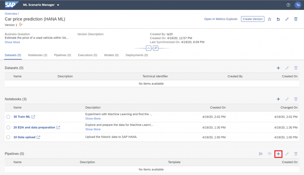
On the ML Scenario’s main page create a new pipeline.
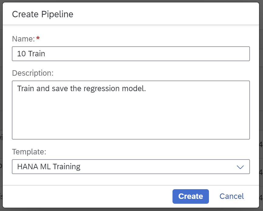
Name the pipeline “10 Train” and select the “HANA ML Training” template. Click “Create”.
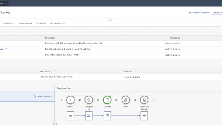
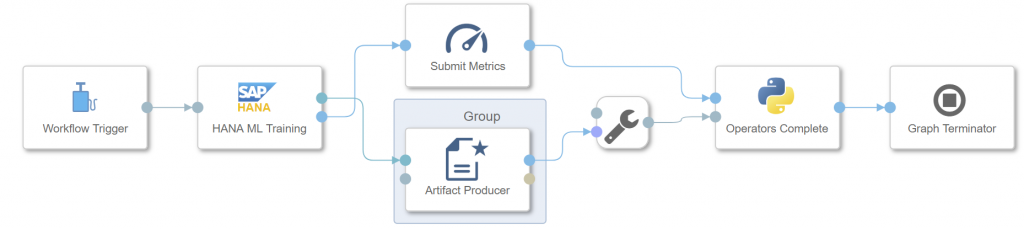
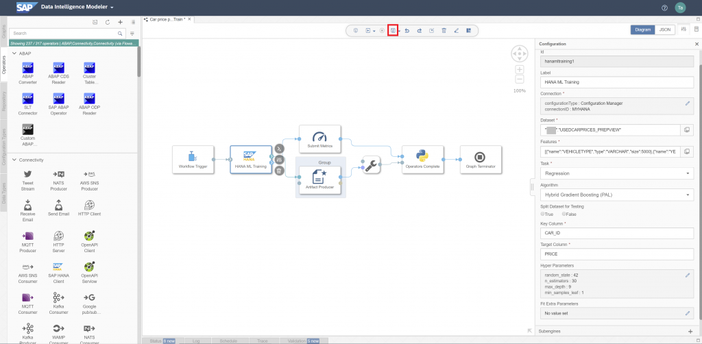
The pipeline opens in the Modeler interface. All operators that we need are already there. The model will be trained through the “HANA ML Training” operator. The operator has two outputs, as it saves the model into the ML Scenario through the “Artifact Producer” and it can also save model metrics (i.e. quality indicators) into the same scenario. Once both branches have completed, the pipeline terminates.
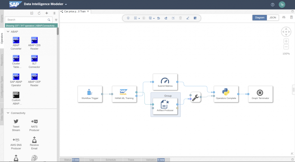
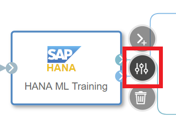
Only the “HANA ML Training” operator must be configured with our requirements. The other operators can remain unchanged. Open the operator”‘s configuration.
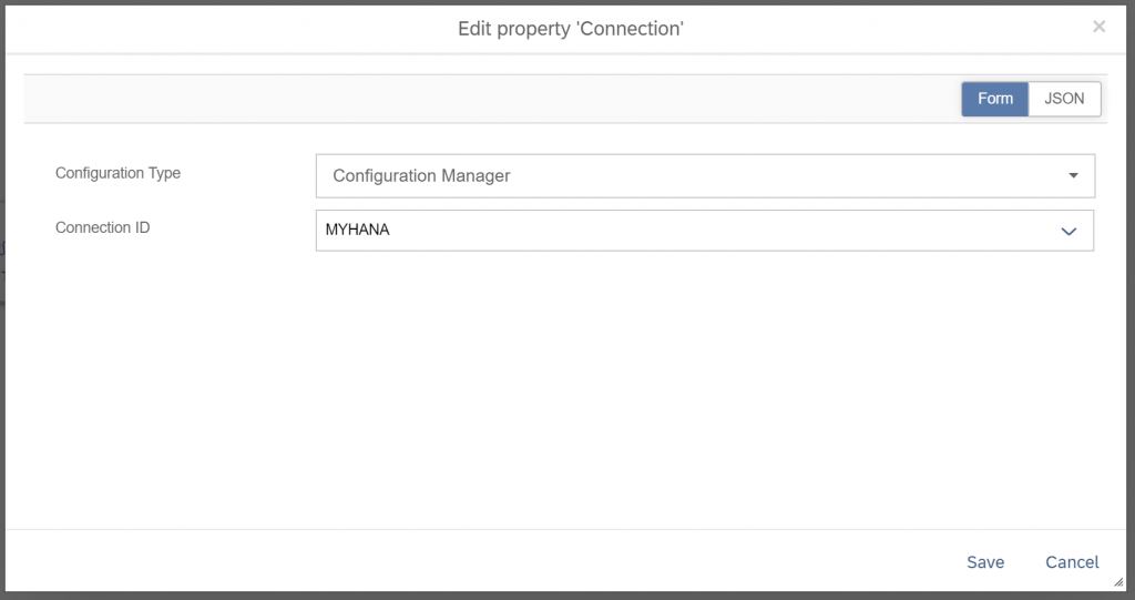
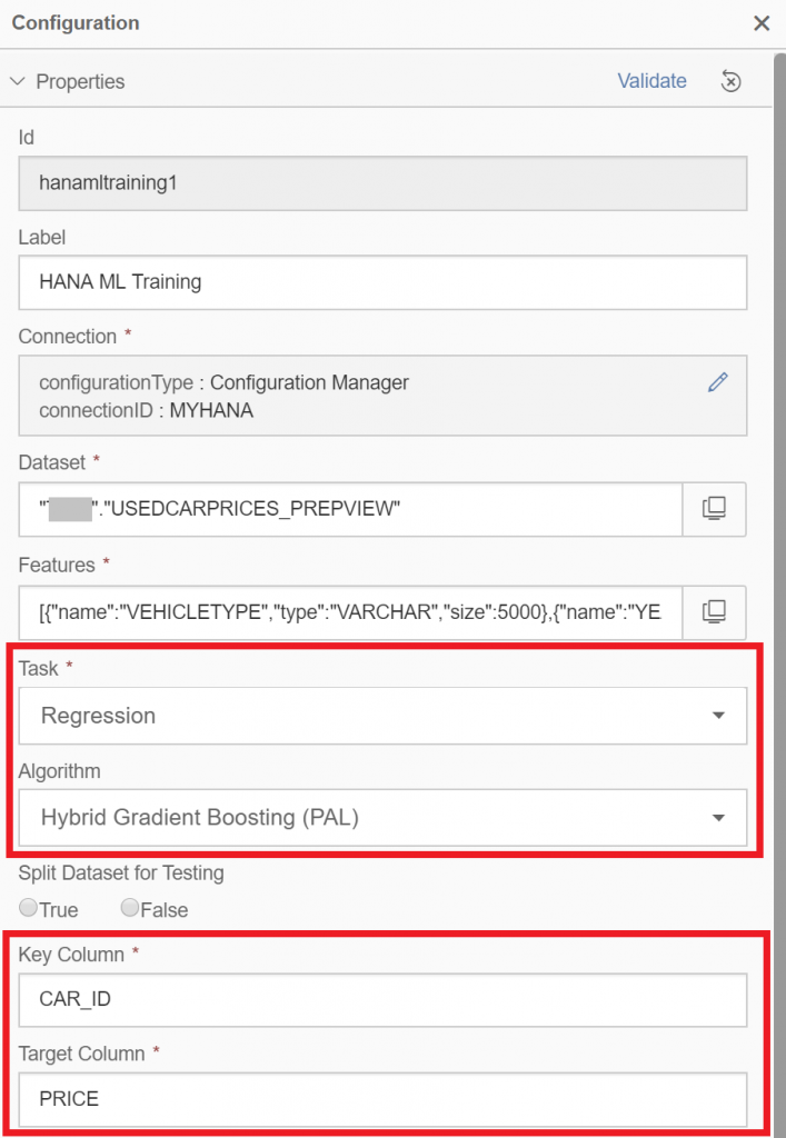
First specify the connection. Set the “Configuration Type” to “Configuration Manager”. Then select the “MYHANA” connection from the “Connection ID” drop-down and save.
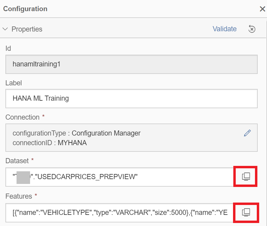
Still in the configurations of the “HANA ML Training” operator, select as “Dataset” the “USEDCARPRICES_PREPVIEW” in your schema, which provides the data in the format needed to train the model. In the Features section, remove the “CAR_ID” and “PRICE” columns. The ID and target should always be explicitly excluded.
Specify the algorithm by setting the “Task” drop-down to “Regression”, then select “Hybrid Gradient Boosting (PAL)” as algorithm. Manually enter the “Key Column” as “CAR_ID” and the “Target Column” is “PRICE”.
Now specify the algorithm’s hyperparameters, which we found earlier on, that produced the strongest model. Edit the “Hyper Parameters” and enter the JSON syntax below, which specifies our preferred hyperparameters.
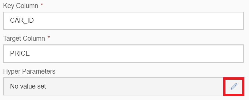
{
“random_state”: 42,
“n_estimators”: 30,
“max_depth” : 9,
“min_samples_leaf” : 1
}
The pipeline is configured. Hit the “Save” icon on top.
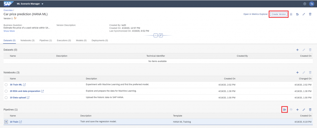
Optionally, in the ML Scenario’s main page you can click “Create Version” at the top of the screen. This creates a new version, which includes all the changes made to the project since the scenario was created. This step used to be compulsory in earlier versions of SAP Data Intelligence, now it is optional.
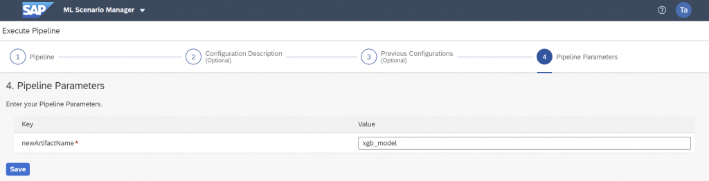
Whether you have created a new version or not, select the “10 Train” pipeline and press the “Execute” button to run the pipeline.
Skip through the settings that appear until the “Pipeline Parameters” are prompted. Set “newArtifactName” to “xgb_model”. The trained model will be saved with this name in the ML Scenario. Then click outside the parameter box, so that the “Save” option appears, which you click.
After a short while the execution’s summary screen shows that the pipeline completed successfully. No metric is shown, as we hadn’t specified a test set in the “HANA ML Training” operator.
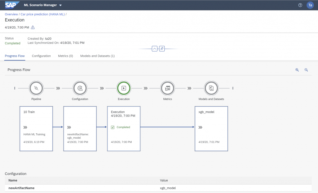
The model is saved in the ML Scenario and can be used for predictions through an inference pipeline.
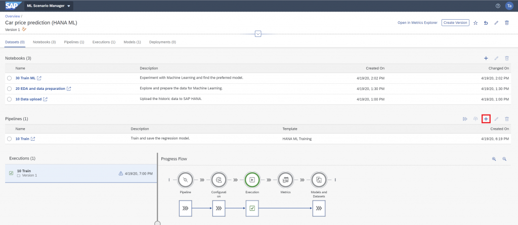
Inference pipeline
Create this second and final pipeline in the ML Scenario’s main page.
Name the pipeline “20 Real-time prediction” and choose the “HANA ML Inference” template.
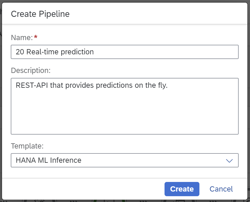
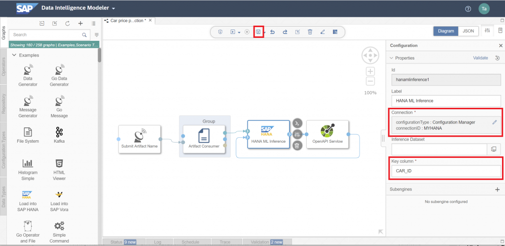
This inference pipeline looks rather different to the training pipeline, as it serves a very different purpose. This pipeline is supposed to run permanently. The “OpenAPI Servlow” operator provides a REST-API, which can be called to obtain a prediction. That prediction is carried out through the model that was saved with the “10 Train” pipeline.
Quickly configure this pipeline. You only need to set the “Connection” to “MYHANA” as before. And set the “Key column” to “CAR_ID”. Then hit the “Save” icon at the top.
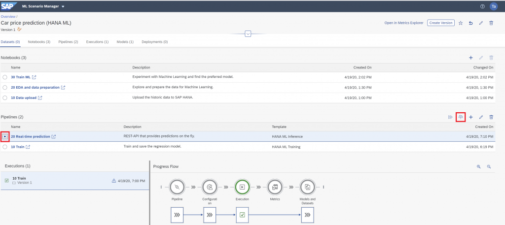
Select the new pipeline on the ML Scenario’s main page and click the “Deploy” icon.
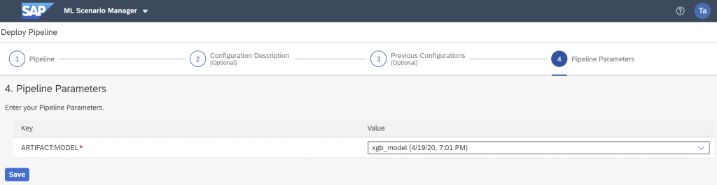
Click through the options that come up until you can select the trained model from a drop-down. This model appears here, because it had been saved into the ML Scenario by our training pipeline. Continue with “Save”.
After a short while the pipeline should be “Running”. The “Deployment URL” shows the base path under which the pipeline can be called. Click the icon to the right of the URL to copy the address.
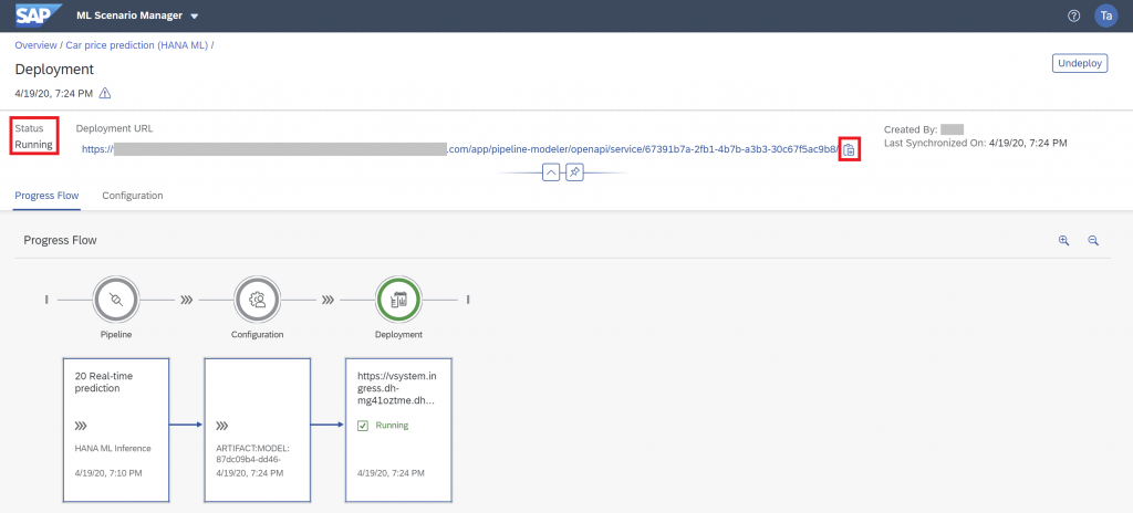
The pipeline is running and ready to provide predictions in real-time.
Real-time prediction
Let’s predict the price of the car!
Keep the Deployment URL from the previous step, you will need it soon. First however install a program to test the REST-API. You can use any tool you like that can call a REST-API. I will be using Postman. Just follow the link and download and install. This should all be possible without having to register anywhere.
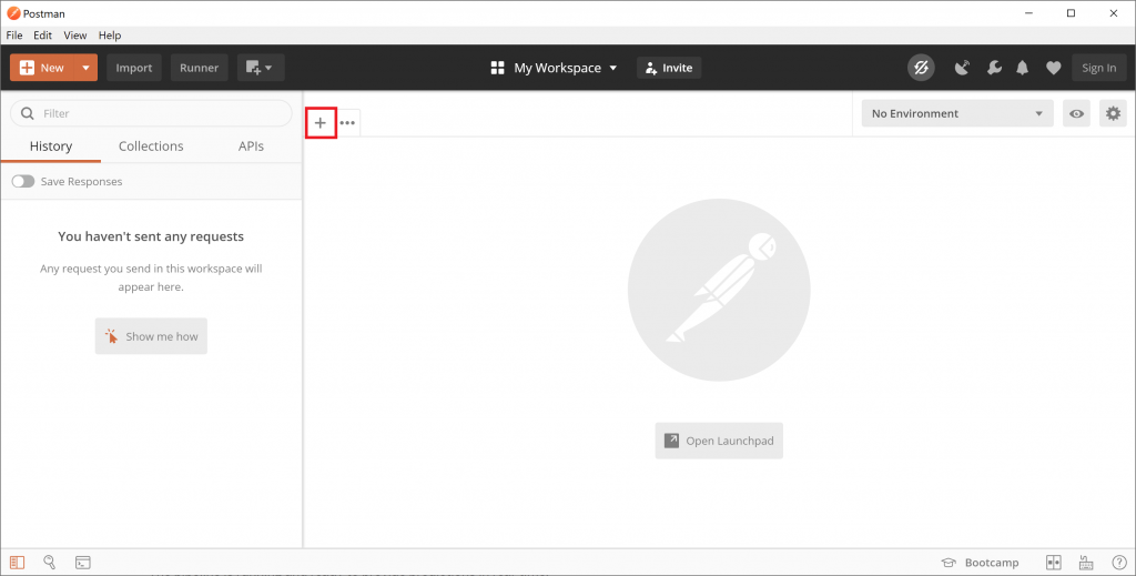
Open Postman and create a new “Request” with the little “+” icon.
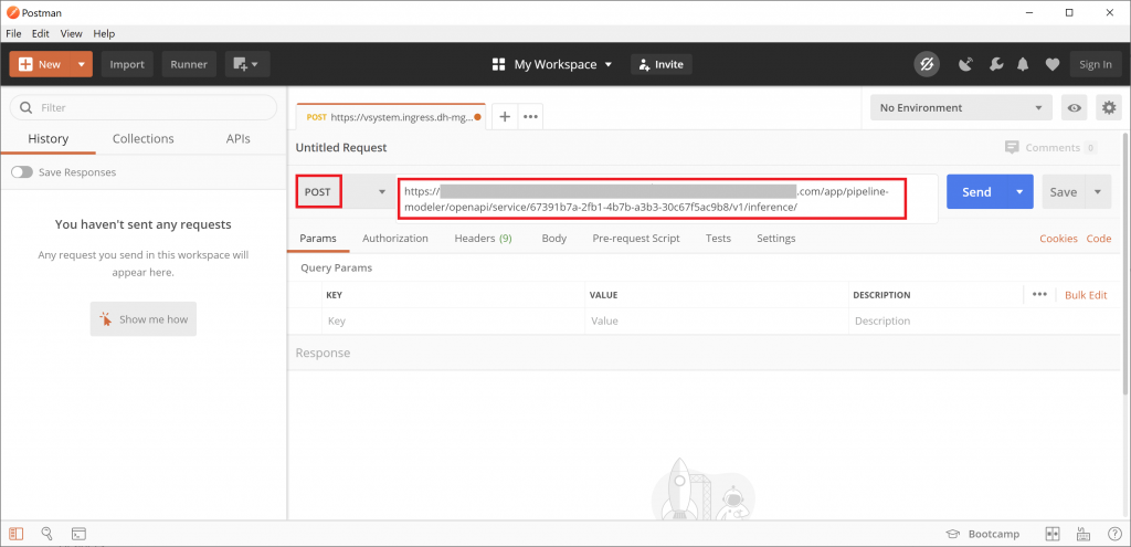
Copy the “Deployment URL” into the address bar that opened up. Extend this address by adding “v1/inference/” at the end. Also change the drop-down of the request type from “GET to “POST”.
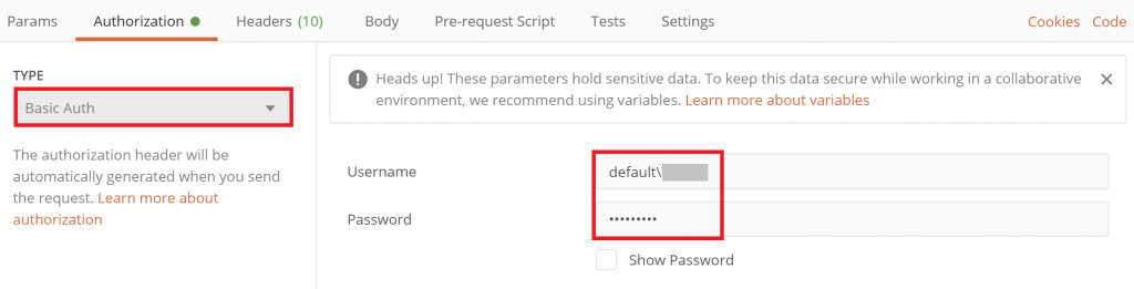
Go into the “Authorization” tab and set the “TYPE” to “Basic Auth”. Enter the username, which is the name of the tenant of SAP Data Intelligence, followed by “\” and your username. If you are working in the default tenant with user DS, you need to enter default\DS. Don’t forget to enter the password.
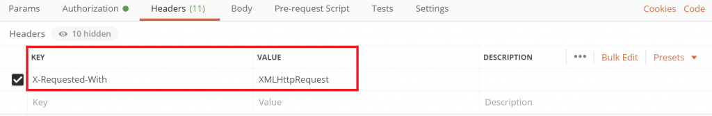
On the “Headers” tab, add the following entry:
- Key: X-Requested-With
- Value: XMLHttpRequest
And finally, in the “Body” tab specify the car, for which you want a price prediction. Select “Raw” and enter this JSON syntax.
{
"CAR_ID" : [1],
"VEHICLETYPE" : ["coupe"],
"YEAR" : [2010],
"GEARBOX" : ["manual"],
"HP" : [120],
"MODEL" : ["C-Class"],
"KILOMETER" : [40000],
"FUELTYPE" : ["petrol"]
}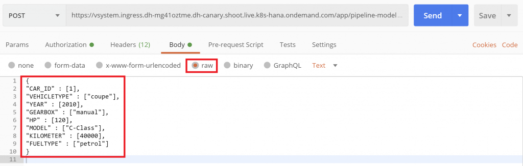
All that’s left, is to click the “Send” button.
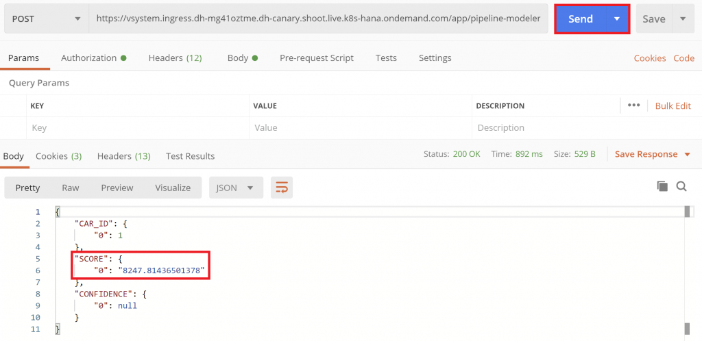
Lo and behold, we have a prediction! The score is the price the model estimates for our imaginary car. Try out different specifications, i.e. different values for the kilometers, and see how the predictions change.
With the REST-API now providing the predictions, business applications can make use of them in real-time. This video shows an example of a chatbot, which uses a similar REST-API from SAP Data Intelligence to provide car price estimates. The model behind this chatbot is a little simpler, it only requires the car’s model, the year in which it was built, and the car’s mileage.


