REQUIREMENT
This blog is regarding the calculation of “Production Ratio” in Supply Chain Management for the monthly bucket in SAP HANA.
The client wanted to see, Production Ratio of a year for each month for a particular Product, Location and Product Version combination. In my case Production Ration was calculated as (Quantity / Total Quantity * 100) for each month. The catch is when there is no value for Quantity and Totaly Quantity in a month, then we have to look forward to the upcoming months for values.
Use Case: Reapplying the production/ transportation quota to most relevant BOM/ lane. This scenario is applicable in almost all the supply chain planning projects where you take constrained/ unconstrained supply plan and extracts production and transportation quotas for Inventory planning.
DATA and SOLUTION
Let me first introduce you with the reference table which has six columns namely PRODUCT, LOCATION, P_VERSION (PRODUCT VERSION), QTY (QUANTITY), TOTAL_QTY (TOTAL QUANTITY) and DATE.
This table contains the list of ordered quantity of a product (i.e. material) from a location (i.e. plant) for an entire year. If you look at the table, there is a zero (or null) quantity ordered in Jan. In Feb, we have ordered 10 quantity of product version 001 and 20 quantity of product version 002, so the total order quantity is 30. Similarly, we have values of ordered quantity for the rest of the months.
Now, when I say we have to look forward whenever there is a null value for QTY and TOTAl_QTY, then for Jan, we should have values from Feb (which is the first non-null value month after Jan) Hence, for Jan there will be two product versions 001 and 002, and their respective ordered quantity from Feb. Similarly, for Mar, Apr, May and June, July is the desired month to look for value.
In simple words,
- Jan will have values from Feb. (two versions)
- Mar, Apr, May and June will have values from July.
- Aug and Sept will have values from Oct. (two versions)
- Nov will have values from Dec.
To achieve this, I have used Table Function, which can be further consumed in a Calculation view to get the result.
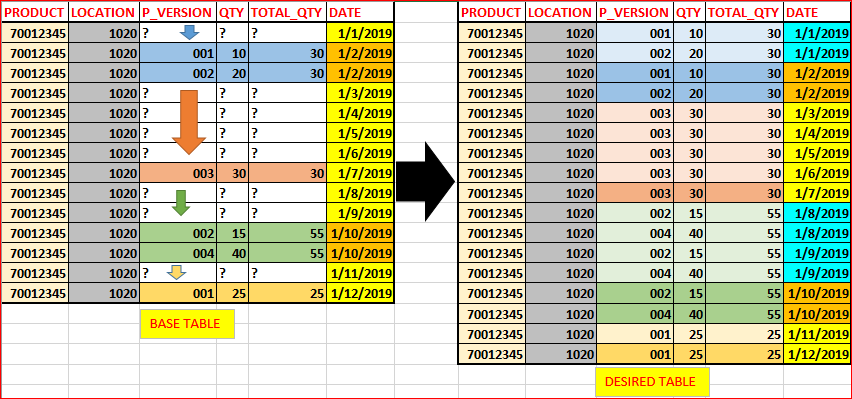
TABLE T1 SELECTING VALUES
Select all the values from the referenced table or VDM.
T1 = Select * From BASE_TABLE;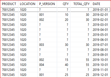
TABLE T2 SET FLAG WHERE TOTAL_QTY IS NULL
Here, we will select only “PRODUCT”, “LOCATION”, “TOTAL_QTY” and “DATE” fields from table T1. Set FLAG as 0, where the value of “TOTAL_QTY” is NULL, else Set FLAG as 1.
T2 =  SELECT
      "PRODUCT",
      "LOCATION",
      "DATE",
      "TOTAL_QTY",
    CASE When "TOTAL_QTY" Is Null
    Then 0
    ELSE 1
    END AS "FLAG"
FROM :T1
order by "DATE";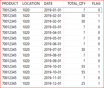
TABLE T3 APPLY RUNNING SUM ON FLAG
Now, apply the “Running Sum” Function on the “FLAG” column. By doing so, you would notice that the value of running sum column, i.e., “FLAG_SUM” changes whenever a non-null “TOTAL_QTY” row occurs. This will become clearer in the next step, how this would help us.
T3 = SELECT
     "PRODUCT",
     "LOCATION",
     "DATE",
     "TOTAL_QTY",
     "FLAG",
     SUM("FLAG") OVER (PARTITION BY "PRODUCT","LOCATION" ORDER BY "DATE") AS "FLAG_SUM"
FROM :T2
order by "DATE";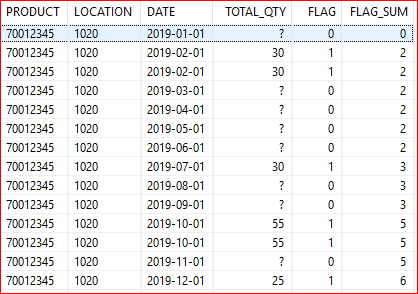
TABLE T4 APPLY ROW_NUMBER() ON FLAG_SUM
Apply ROW_NUMBER() Function on “PRODUCT”, “LOCATION”, and “FLAG_SUM” and Order By “DATE” in DESC order.
Now, if you look at the result, the “ROW_NUM” column gives the number of rows (here, months) to look forward to get the value. For example, the value for Jan is supposed to be picked from Feb. Here, Jan(1) + ROW_NUM(1) = Feb(2). Similarly, for March, April, May and June, the month to look forward for the value is July. So, March(3) + ROW_NUM(4) = July(7), and so on.
NOTE: – ROW_NUMBER() function applied on “DATE” must be in DESC order.
T4 = SELECT
     "PRODUCT",
     "LOCATION",
     "DATE",
     "TOTAL_QTY",
     "FLAG",
     "FLAG_SUM",
     ROW_NUMBER() OVER (PARTITION BY "PRODUCT","LOCATION","FLAG_SUM" ORDER BY "DATE" DESC) AS "ROW_NUM"
FROM :T3
order by "DATE";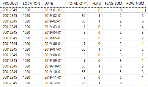
TABLE T5 ADD NUMBER OF MONTHS TO THE DATE COLUMN
Adding the number of months to “DATE” from “ROW_NUM” column to get a new column as “DATE_NEW”, which is the desired month to look forward to the next available value (as explained above).
T5 = SELECT
     "PRODUCT",
     "LOCATION",
     "DATE",
     "TOTAL_QTY",
     "FLAG",
     "FLAG_SUM",
     "ROW_NUM",
      TO_DATE (ADD_MONTHS( "DATE","ROW_NUM")) AS "DATE_NEW"
From :T4
order by "DATE";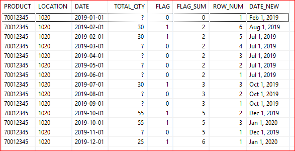
TABLE T6 LEFT OUTER JOIN ON T1 AND T5
Now, apply “Left Outer” join on table T1 and T5, keeping T1 (our base table) as LEFT and T5 (having “DATE_NEW” column) as RIGHT. By this, we will have the desired months to look for under “DATE_NEW” column for each row.
NOTE: – You might have noticed that we are having two rows for P_VERSION-001 in Feb (2019-02-01). These will be handled going forward.
T6 = select
     T1."PRODUCT",
     T1."LOCATION",
     T1."P_VERSION",
     T1."QTY",
     T1."TOTAL_QTY",
     T1."DATE",

     T5."DATE_NEW"

From :T1 AS T1 LEFT OUTER JOIN :T5 AS T5
 on T5."PRODUCT"  = T1."PRODUCT"
AND T5."LOCATION" = T1."LOCATION"
AND T5."DATE"     = T1."DATE"
order by "DATE";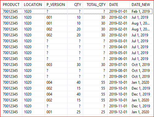
TABLE T7 LEFT OUTER JOIN ON T6 AND T1
Apply “Left Outer” join on table T6 and T1, keeping T6 as LEFT and T1 (our base table) as RIGHT. By this, we will have the desired values of “P_VERSION”, “QTY” and “TOTAL_QTY” under “P_VERSION1”, “QTY1” and “TOTAL_QTY1” columns, respectively, for each row.
NOTE: – As mentioned above, don’t worry about the duplicate entries as we are going to handle them soon.
T7 = SELECT
     T6."PRODUCT",
     T6."LOCATION",
     T6."P_VERSION",
     T6."QTY",
     T6."TOTAL_QTY",
     T6."DATE",

     T1."P_VERSION" AS "P_VERSION1",
     T1."QTY" AS "QTY1",
     T1."TOTAL_QTY" AS "TOTAL_QTY1"

FROM :T6 AS T6 LEFT OUTER JOIN :T1 AS T1
 on T1."PRODUCT"  = T6."PRODUCT"
AND T1."LOCATION" = T6."LOCATION"
AND T1."DATE"     = T6."DATE_NEW"
order by "DATE";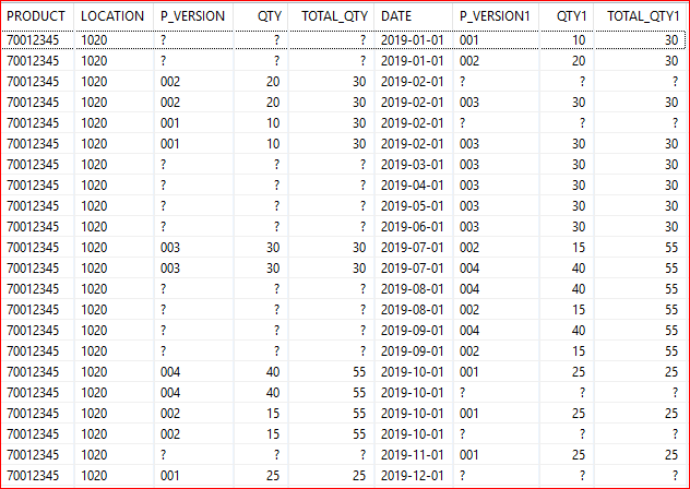
OUTPUT BUILD USING T7
Select the required fields “PRODUCT”, “LOCATION”, “P_VERSION”, “QTY”, “TOTAL_QTY” and “DATE”.
“SELECT DISTINCT” will remove the duplicate entries (as mentioned above).
Now, if we have a null value for “P_VERSION”, only then “P_VERSION1” will be picked up. Else, “P_VERSION” will remain as it is. Similar will be the case for “QTY” and “TOTAL_QTY”. This will give us our final output.
var_out =
   SELECT
	 DISTINCT
	 "PRODUCT",
	 "LOCATION",

	 CASE When "P_VERSION" Is Null
	 Then "P_VERSION1"
	 ELSE "P_VERSION"
	 END AS "P_VERSION",

	 CASE When "QTY" Is Null
	 Then "QTY1"
	 ELSE "QTY"
	 END AS "QTY",

	 CASE When "TOTAL_QTY" Is Null
	 Then "TOTAL_QTY1"
	 ELSE "TOTAL_QTY"
	 END AS "TOTAL_QTY",

	 "DATE"

FROM :T7
order by "DATE",
         "P_VERSION";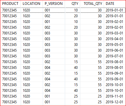
By this, we are having the values of Quantity and Total Quantity for each month which will help us in calculating our Production Ratio for the monthly bucket.


