Why do we need to partition tables in HANA?
As HANA can not hold more than 2 billion records per column store table or per partition, any table which has crossed more than 1.5 billion rows are valid candidates of partitioning. It also helps in parallel procession of queries, if they are distributed across nodes in case of HANA scale out scenario producing results faster.
CASE STUDY: Here I am going to change an existing table which is partitioned on all the key fields to partition on 1 optimum key column: ie, The partition of a table EDIDS is going to be changed from HASH 21 MANDT, DOCNUM, LOGDAT, LOGTIM, COUNTR to HASH 7 DOCNU. The main reason is because, many SQLs and joins that are running against this table are running with where clause on DOCNUM.
Steps:
Log into studio and display the table and make a note of details.
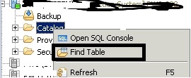
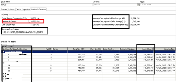
Find the table and display: Observe the things highlighted below. Column Key: Primary key fields of any table.

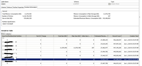
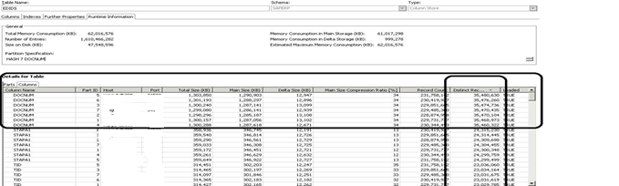
Check the runtime properties.:
Things to observer here.
Number of entries =Row count(3.1 billion)
Memory consumption in main and in Delta is also indicated there.
Partition specification: 21 partitions distributed across 7 slave nodes, 3 partitions per node.
So how does HANA handles this partitioning?
When the alter command specified in previous gets executed below things happen in backend in HANA DB.
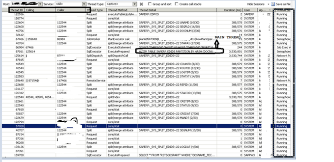
We can check for the status of the threads from performance tab and filter it out based on the master node and into the server on which this table is sitting.
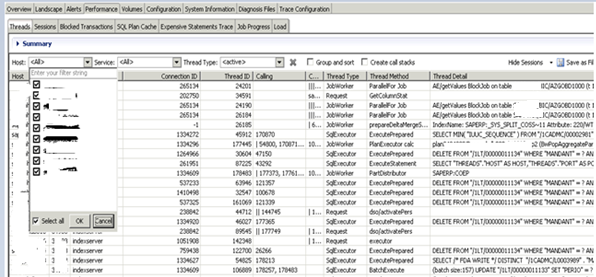
Look for the SQL that we had executed: Choose the master node and the slave node to which we had moved the partitions to.
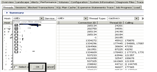
Click ok.
Sort by application user in performance tab. Though I had logged in as SYSTEM for re-partition, HANA will also know the WTS via which I am connecting to this DB.
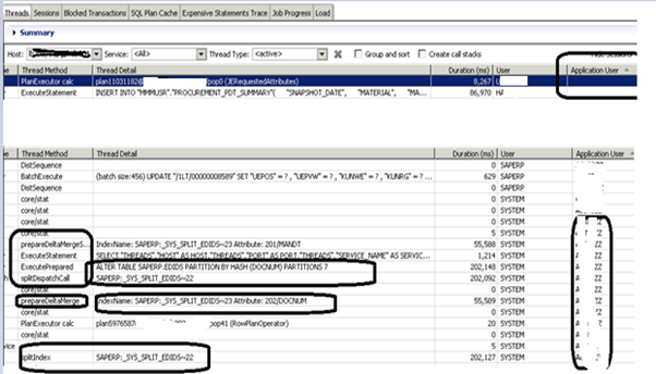
In the background
1. My SQL gets prepared and delta merge for that table will first executed.
Here is my delta merge job that got triggered and the other jobs that will follow the same.
Below delta merge job has got completed 59/63. All the remaining jobs has 30 steps and it will run in parallel post delta merge completes.
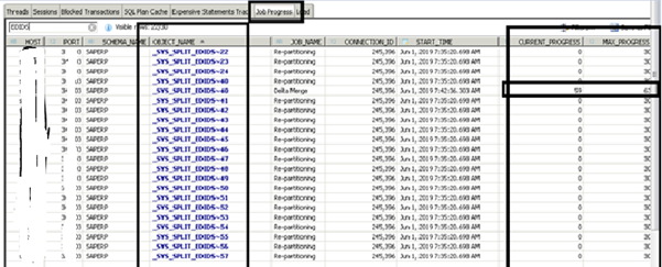
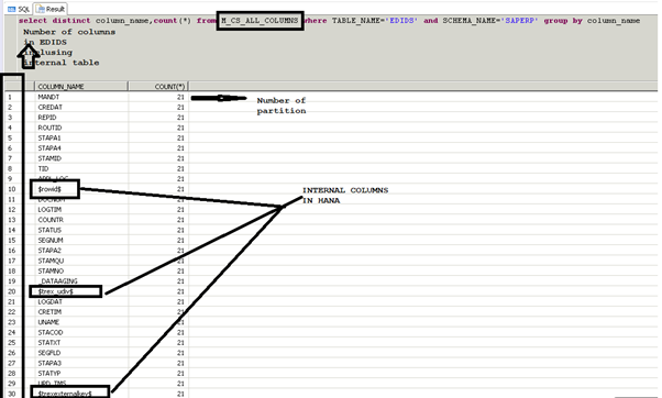
so, Why is the max progress for _SYS_SPLIT_EDIDS shows as 30 ? It is actually the total number of columns in that table (including internal columns)
I have used M_CS_ALL_COLUMNS rather than M_CS_COLUMNS because the former also holds hana internal columns against the lateral
Lets check the threads now.
After 6 hours, my re-partition got completed. Now I distribute the 7 partitions between the 7 HANA nodes. Moving back the partitions:
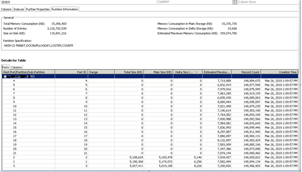
Post re-partition and table distribution to different nodes.
Here if we see the total 3.1 billion is spread across 21 partitions with around 148 million records count per partition.
To partition command to work, we need to first move all the partitions from different node to single node.
Below I choose a to leave partitions 1, 2, 3 to the same server and move the other partitions from other servers to this server.
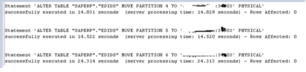
Sample SQL:
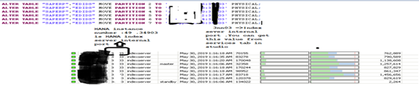
ALTER TABLE “SAPERP”.”EDIDS” MOVE PARTITION 4 TO ‘<server_name>:3<nn>03’ PHYSICAL;

ALTER TABLE “SAPERP”.”EDIDS” MOVE PARTITION 5 TO ‘<server_name>:3<nn>03’ PHYSICAL;

ALTER TABLE “SAPERP”.”EDIDS” MOVE PARTITION 6 TO ‘<server_name>:3<nn>03’ PHYSICAL;

ALTER TABLE “SAPERP”.”EDIDS” MOVE PARTITION 7 TO ‘<server_name>:3<nn>03’ PHYSICAL;

ALTER TABLE “SAPERP”.”EDIDS” MOVE PARTITION 8 TO ‘<server_name>:3<nn>03’ PHYSICAL;

ALTER TABLE “SAPERP”.”EDIDS” MOVE PARTITION 9 TO ‘<server_name>:3<nn>03’ PHYSICAL;

ALTER TABLE “SAPERP”.”EDIDS” MOVE PARTITION 10 TO ‘<server_name>:3<nn>03’ PHYSICAL;

ALTER TABLE “SAPERP”.”EDIDS” MOVE PARTITION 11 TO ‘<server_name>:3<nn>03’ PHYSICAL;

ALTER TABLE “SAPERP”.”EDIDS” MOVE PARTITION 12 TO ‘<server_name>:3<nn>03’ PHYSICAL;

ALTER TABLE “SAPERP”.”EDIDS” MOVE PARTITION 13 TO ‘<server_name>:3<nn>03’ PHYSICAL;

ALTER TABLE “SAPERP”.”EDIDS” MOVE PARTITION 14 TO ‘<server_name>:3<nn>03’ PHYSICAL;

ALTER TABLE “SAPERP”.”EDIDS” MOVE PARTITION 15 TO ‘<server_name>:3<nn>03’ PHYSICAL;

ALTER TABLE “SAPERP”.”EDIDS” MOVE PARTITION 16 TO ‘<server_name>:3<nn>03’ PHYSICAL;

ALTER TABLE “SAPERP”.”EDIDS” MOVE PARTITION 17 TO ‘<server_name>:3<nn>03’ PHYSICAL;

ALTER TABLE “SAPERP”.”EDIDS” MOVE PARTITION 18 TO ‘<server_name>:3<nn>03’ PHYSICAL;

ALTER TABLE “SAPERP”.”EDIDS” MOVE PARTITION 19 TO ‘<server_name>:3<nn>03’ PHYSICAL;

ALTER TABLE “SAPERP”.”EDIDS” MOVE PARTITION 20 TO ‘<server_name>:3<nn>03’ PHYSICAL;

ALTER TABLE “SAPERP”.”EDIDS” MOVE PARTITION 21 TO ‘<server_name>:3<nn>03’ PHYSICAL;
o/p:
Post this we have all the partition in one node in a scale out environment.
Now I proceed with partitioning command.
ALTER TABLE SAPERP.EDIDS PARTITION BY HASH (DOCNUM) PARTITIONS 7;

DETERMINING THE OPTIMUM COLUMN and NUMBER FOR PARTITION
So why would I consider DOCNUM as optimal column to be partitioned and why the number of partitions was choosen as 7?
In order to choose a column for partitioning we need to analyze the table usage in depth.
Analyzing and understanding the SQLs on the table:
1. Check with the functional team. Ask them which column does they query frequently and which column is always part of where clause. If they are not very clear on the same we can help them with plan cache data.
Eg: If a table keep getting queried based on a where clause on year, and in general the table has data since 2015, a Range partition on YEAR column will create a clear demarcation between hot and cold data.
Sample SQL for range partition:
ALTER TABLE SAPERP.BSEG PARTITION BY RANGE (BUKRS) (PARTITION 0 <= VALUES < 1000, PARTITION 1000 <= VALUES < 1101, PARTITION 2000 <= VALUES < 4000,PARTITION 4000 <= VALUES < 4031, PARTITION 4033 <= VALUES < 4055, PARTITION 4058 <= VALUES < 4257, PARTITION VALUE = 4900, PARTITION OTHERS);2. Check M_SQL_PLAN_CACHE.
With the help of below query we can get a list of queries that are to identify the where clause
select statement_string, execution_count, total_execution_time from m_sql_plan_cache where statement_string like ‘%<TABLE_NAME>%’ order by total_execution_time desc;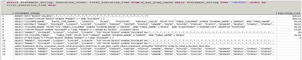
3. How to check the columns that are getting joined on this table using Join statistics?
Download the SQL HANA_SQL_Statistics_JoinStatistics_1.00.120+ from OSS 1969700 and modify the SQL like below.
Goto modification section.
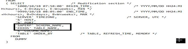
Modify the modification section as per your requirement.
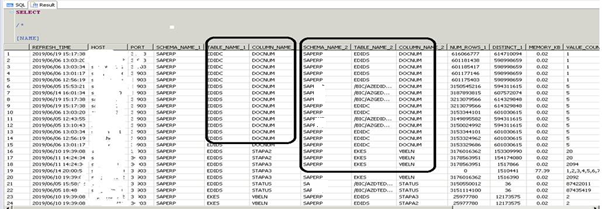
From above we can see that most of the joins are happening on DOCNUM and hence a HASH on this column will make the query runtime faster.
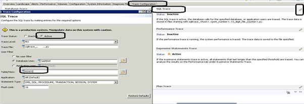
4. There can be some cases where we will not have enough information even from here or it will be empty. In that case we will have to enable the sql trace for the specific table.
5. If there is no specific range values that are frequently queried and if we have a case like most of the columns are used most of the times a HASH algorithm will be a best fit.
It is similar to round robin partition but, data will be distributed according to the hash algorithm on their one or 2 designated primary key columns.
– A Hash algorithm can only happen on a PRIMARY key field.
– It is always optimal not to choose more than 2 primary key field for HASH
– Within primary key, check for which row has maximum distinct records. That specific column can be chosen for re-partition.
To determine which primary key column we can choose for re-partition, perform below.
a. Load the table fully into memory

b. Open the table from studio and find the primary key for the table
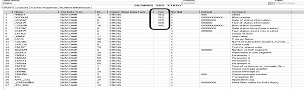
c. Find the primary key column which has maximum distinct record.
Hence a HASH on DOCNUM for EDIDS table is best choice.
ALTER TABLE SAPERP.EDIDS” PARTITION BY HASH (DOCNUM) PARTITIONS 7
NOTE: When ever a table is queried and if that table or partition is not present in memory HANA automatically loads it into the memory either partially or fully. If that table is partitioned, which ever row that is getting queried, then that specific partition which has the required data gets into memory. Even if you only need 1 row from a partition of a table which has 1 billion records, that entire partition will get loaded either partially or fully. In HANA we can never load 1 row alone into memory from a table.
So, How to determine the number of partitions in scale out scenario?
The optimal number of partition should be decided optimally such that the load gets distributed across different nodes in HANA in case of scale-out scenario.For a table which is not yet partitioned and which is nearing more than 1.5 billion.
It is recommended to always go for n-1 number of partition where n is the total number of nodes in HANA including Master node. Why -1 is because we should not have any partitions sitting on master node as it will always be better to leave the master node alone to perform transaction processing alone.
Eg:
HANA – 1 master node, 3 slaves, 1 standby => Then the number of partitions is 3. (Always don’t take into count the standby node as it does not have any data volumes assigned to it)
HANA – 9 nodes =1 Master, 7 slaves, 1 standby =>Partition number should be 7 and it should be distributed across the worked nodes via the move command specified
GENERAL RULE OF THUMB IN PARTITION
– We can have any number of partitions as you specify, but it is generally not advisable to have any tables with more than 100 partitions
– It is recommended to have atleast 100 million records per partitions and each partition memory utilization at any point of time should not be more than 50GB.
– Any non-partitioned table which has more than 2.14 billion records will make the system crash and hence it is best to put a partition when it is at 1.5 billion
– For tables which are already partitioned and we have to re-partition as either the current partition is not optimal or if the record count per partition is more than 1.5 billion we need to increase the number of partitions
– Always choose the number of partition as a multiple or dividend of current partition. Eg:If a table is partitioned with 7 partition, you can increase the partition to 7*2=14 or so on. This is only useful to make the partition job run parallelly.
– HANA will crash if the number of rows per partition is more than 2.14 billion
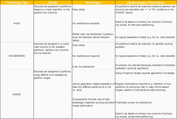
TYPES OF BASIC PARTITIONS AND THEORY INVOLVED
- The partitioning feature of the SAP HANA database splits column-store tables horizontally into disjunctive sub-tables or partitions. In this way, large tables can be broken down into smaller, more manageable parts. Partitioning is typically used in multiple-host systems.
- HANA can not hold any table which is not partitioned to have more than 2.14 billion records. To overcome this limitation re-partitioning of tables comes into picture along with enhancing the query performance in a scale -out scenario.
- There are certain reasons for splitting tables in multiple partitions:
- To improve performance on delta merge operations
- If the WHERE clause of a query matches the partitioning criteria, then it may be possible to exclude some partitions from the execution of the query or even to execute it on a single partition only
- To avoid running into limitation of storing maximum 2 billion rows
- For load balancing in scale-out environments
- To improve performance on delta merge operations
- AP HANA provides administration tools for monitoring table distribution and redistributing tables. There are table placement rules that are used to assign certain tables always to the master or to slave index servers, or to specify the number rows that should trigger a repartitioning of the table. Table placement rules are created based on a classification of tables into table group types, sub types and groups, which is part of the table metadata.
NOTE: 1. If we have primary key fields we can use only HASH or RANGE. 2. ROUNDROBIN can only be used when we don’t have any primary key fields. 3. RANGE PARTITION can not be based on non primary key fields. 4. HASH partition can only be done on primary key fields like range partition. 5. HASH algorithm is based on primary key fields which has maximum number of distinct records as already discussed which can be determined after loading the table into memory. 6. We can find the most frequently ran SQL on any table from M_SQL_PAN_CACHE as shown which might also help in determining the best algorithm based on “WHERE” clause in SQL. select statement_string, execution_count, total_execution_time from m_sql_plan_cache where statement_string like ‘>table_name>%’ order by total_execution_time desc; HANA Partitioning- Partitioning Performance Tips
Consider the following possible optimization approaches:
- Make sure that existing partitioning optimally supports the most important SQL statements
- Define partitioning on as few columns as possible
- Use as few partitions as possible
- Try to avoid changes of records that require a remote uniqueness check or a partition move
- For HASH partitioning, include at least one of the key columns
- Starting with SAP HANA 1.00.122 OLTP accesses to partitioned tables are executed single-threaded and so the runtime can be increased compared to a parallelized execution (particularly in cases where a high amount of records is processed). You can set indexserver.ini -> [joins] -> single_thread_execution_for_partitioned_tables to ‘false’ in order to allow also parallelized processing (e.g. in context of COUNT DISTINCT performance on a partitioned table). See SAP Note 2620310 for more information.
- The partitioning process can be parallelized using parameters below(Note 2222250:For Split_threads parameter, value=80 would be a good starting value for production system. You can consider to increase until 128 based on system behavior.
- To avoid transaction timeouts during long running partitioning SQL statements, please increase timeout parameters. (See Note 1909707)
- The partitioning process can be parallelized using parameters below(Note 2222250:For Split_threads parameter, value=80 would be a good starting value for production system. You can consider to increase until 128 based on system behavior.
indexserver.ini -> [transaction] -> idle_cursor_lifetime
SQL COMMANDS FOR PARTITIONING:1.RANGE:
Sample SQL: ALTER TABLE SAPERP.BSEG PARTITION BY RANGE (BUKRS) (PARTITION 0 <= VALUES < 1000, PARTITION 1000 <= VALUES < 1101, PARTITION 2000 <= VALUES < 4000,PARTITION 4000 <= VALUES < 4031, PARTITION 4033 <= VALUES < 4055, PARTITION 4058 <= VALUES < 4257, PARTITION VALUE = 4900, PARTITION OTHERS);
We have to be very cautious with the range that we choose in range partition. Range partition will not ensure equal distribution of data. Eg. In above query we have a range as below
PARTITION 1 = BUKRS->1 to 999
PARTITION 2 = BUKRS->1000 to 1100
PARTITION 3 = BUKRS->2000 to 3999
PARTITION 4 = BUKRS->4000 to 4030
PARTITION 5 = BUKRS->4033 to 4054
PARTITION 6 = BUKRS->4058 to 4256
PARTITION 7 = BUKRS = 4900
PARTITION 8 = BUKRS-> Any other value
We have dedicated 1 full partition to value BUKRS=4900 as it alone will have around 400 million records. In above we have chosen a range where each partition will have around 300 to 400 million records. Any other value for BUKRS will go and sit in PARTITION 8. However we need to be very careful on the range because any new inserts will go into only partition 8 and we should ensure that its row count does not gets overloaded.
A wise use of range partition will ensure a good separation between hot and cold data.
2. ROUNDROBIN:
SQL:
ALTER TABLE SAPERP.”/BIC/FZGFSMT02″ PARTITION BY ROUNDROBIN 7
Here for round robin, a primary requirement is that they do not have any primary key fields. In that case a roundrobin with 7 partition will ensure data inserts in all the partition in cyclic manner.
Row 1 will go to partition 1
Row 2 will go to partition 2
Row 3 will go to partition 3
Row 3 will go to partition 4
Row 3 will go to partition 5
Row 3 will go to partition 6
Row 3 will go to partition 7
Row 3 will go to partition 1
Row 3 will go to partition 2
….. and so on.
MULTILEVEL-PARTITIONING:
What is multi-level partitioning?Multi-level partitioning can be used to overcome the limitation of single-level hash partitioning and range partitioning, that is, the limitation of only being able to use key columns as partitioning columns. Multi-level partitioning makes it possible to partition by a column that is not part of the primary key.
There are 4 types of multi-level partitioning.
1. HASH-RANGE – Most common
2. Round_Robin-RANGE
3. Hash-Hash
4. RANGE-RANGE
SAMPLE Commands:
1. HASH-RANGE partition: ALTER TABLE SAPERP.CDPOS_RANGE1 PARTITION BY HASH (a, b) PARTITIONS 4,RANGE (c) (PARTITION 1 <= VALUES < 10, PARTITION 10 <= VALUES < 20)

2. Round_Robin-RANGE partition:ALTER TABLE SAPERP.CDPOS_RANGE1 PARTITION BY ROUNDROBIN PARTITIONS 4,RANGE (c) (PARTITION 1 <= VALUES < 10, PARTITION 10 <= VALUES < 20) or

ALTER TABLE SAPBE3.”/BIC/F****RC002″ WITH PARAMETERS (‘PARTITION_SPEC’ = ‘ROUNDROBIN 5; RANGE KEY_Z***002P 0,1,2,*’);

3. HASH-HASH: ALTER TABLE SAPERP.CDPOS_RANGE1   PARTITION BY HASH (a, b) PARTITIONS 4, HASH (c) PARTITIONS 7

4. RANGE-RANGE:  ALTER TABLE SAPERP.CDPOS_RANGE1  PARTITION BY RANGE (a) (PARTITION 1 <= VALUES < 5, PARTITION 5 <= VALUES < 20), RANGE (c)(PARTITION 1 <= VALUES < 5,  PARTITION 5 <= VALUES < 20)
A. HASH-RANGE:
You can use this approach to implement time-based partitioning, for example, to leverage a date column and build partitions according to month or year. The performance of the delta merge operation depends on the size of the main index of a table. If data is inserted into a table over time and it also contains temporal information in its structure, for example a date, multi-level partitioning may be an ideal candidate. If the partitions containing old data are infrequently modified, there is no need for a delta merge on these partitions: the delta merge is only required on new partitions where new data is inserted. Using time-based partitioning in this way the run-time of the delta merge operation remains relatively constant over time as new partitions are being created and used.As mentioned above, in the second level of partitioning there is a relaxation of the key column restriction (for hash-range, hash-hash and range-range).
B. ROUND-ROBIN-RANGE: Round-robin-range multi-level partitioning is the same as hash-range multi-level partitioning but with round-robin partitioning at the first level.
C. HASH-HASH: Hash-hash multi-level partitioning is implemented with hash partitioning at both levels. The advantage of this is that the hash partitioning at the second level may be defined on a non-key column.
RANGE-RANGE: Range-range multi-level partitioning is implemented with range partitioning at both levels. The advantage of this is that the range partitioning at the second level may be defined on a non-key column.


