Learn how a SAC Planning model can be populated with data coming from custom calculations or Machine Learning. We describe this concept in a series of three blogs.
The blogs in the series are:
- Accessing planning data with SAP Datasphere
- Create a simple planning model in SAC
- Make the planning data available in SAP Datasphere, so that it can be used by a Machine Learning algorithm
- Create a simple planning model in SAC
- Creating custom calculations or ML [coming soon]
- Define the Machine Learning Logic
- Create a REST-API that makes the Machine Learning logic accessible for SAC Planning
- Define the Machine Learning Logic
- Orchestrating the end-to-end business process [coming soon]
- Import the predictions into the planning model
- Operationalise the process
- Import the predictions into the planning model
Note: The hyperlinks to the other blogs of this series and to the sample repository might not yet be working for you. They will be updated as soon as those links are public / permanent.
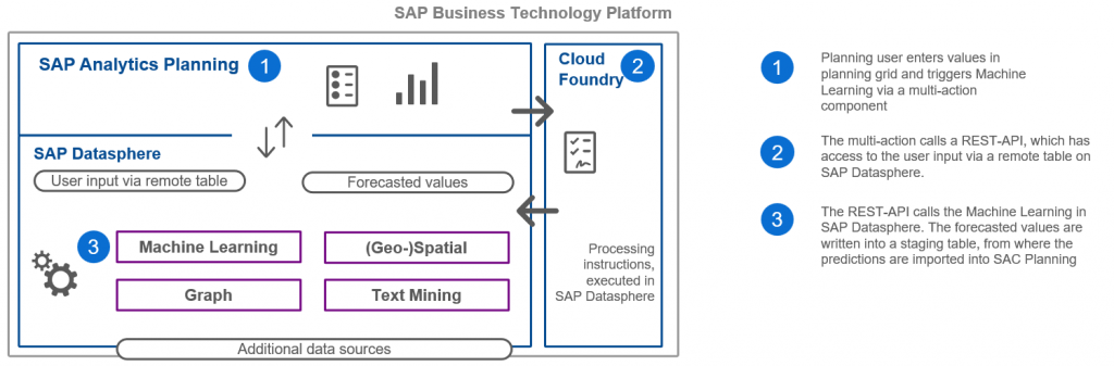
This diagram shows the architecture and process from a high level:
Intro
In the current blog, ‘Accessing planning data with SAP Datasphere’ we will achieve the following tasks:
- create a simple P&L model in SAC and add some data to it
- expose the data in the P&L model in DataSphere
In order to complete the steps described, you will need:
- an SAP Analytics Cloud (SAC) instance
- an SAP Datasphere instance
- a Data Provisioning Agent (DP Agent) set up in your Datasphere instance
1. Create a simple P&L model
1.1 Prepare the data
We will implement the following P&L model:
- Profit = Revenue – Cost
- Revenue = UnitsSold * UnitPrice
- Cost = DirectCost + IndirectCost
- DirectCost = UnitsSold * UnitCost
UnitsSold, UnitPrice, UnitCost and IndirectCost are all inputs to the model
We have to consider two types of data:
- actuals: this is input data that we record about the past
- planning: this is input data that we create for the future
In the current example, we will create:
- 12 months of planning data: 202301 to 202312
- 15 months of actuals data: 202201 to 202303
Then, we will use the actuals for UnitPrice and UnitsSold and the plan for UnitPrice to estimate the plan for UnitsSold via external ML.
We prepare this data in csv and will later upload it to the SAC Planning model.
The data for one month looks like this:
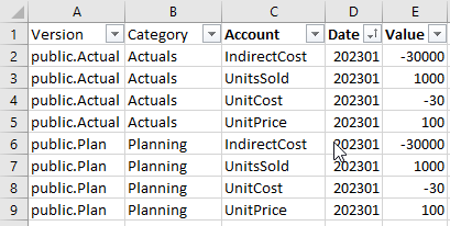
Note that the costs are recorded as negatives. This is to allow hierarchical aggregation.
1.2 Define the model in SAC
This sections assumes some basic familiarity with the SAC interface – so we won’t add screenshots with the location of the required buttons.
We start with an empty model (Modeler -> Create new model -> New Model). This is a planning model by default.
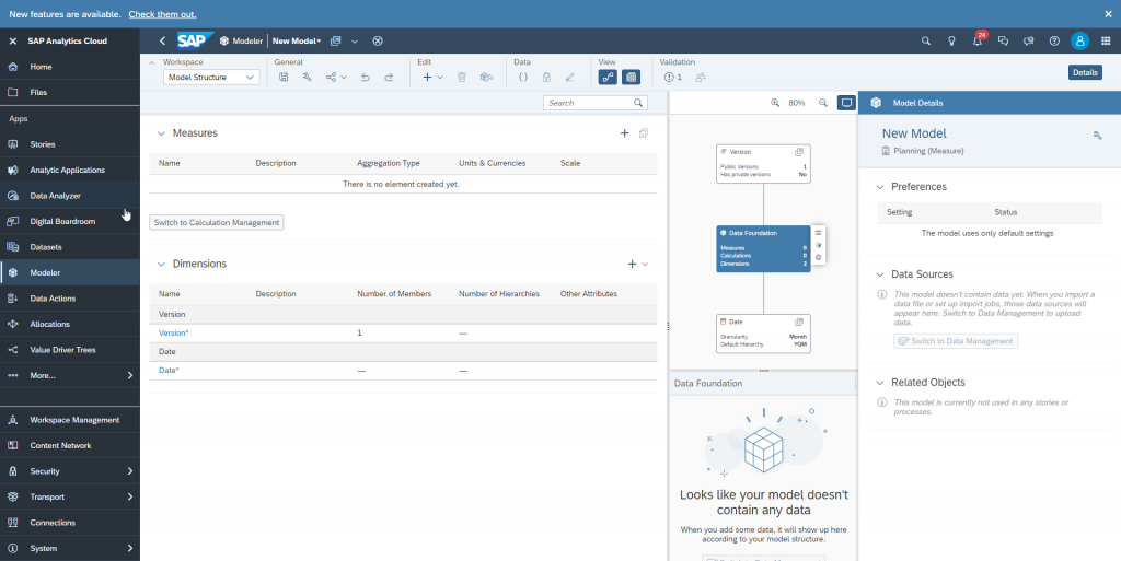
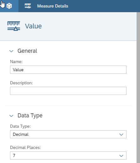
We need one measure which we name ‘Value’ and keep the default decimal type. This will hold the data values.
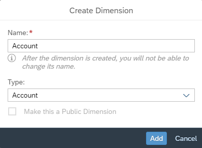
We need one dimension, ‘Account’. Here we will add members for all the different elements in the P&L model.
The dimension type is ‘Account’. This will create a hierarchy allowing us to aggregate accounts hierarchically.
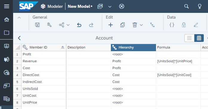
We add all the elements of the P&L as members of the Account dimension and specify how the computations take place (i.e. we implement the calculation model).
- Profit and Cost will be computed by aggregation along the hierarchy (the ‘Hierarchy’ column specifies the element that the current element aggregates into)
- Revenue and DirectCost will be computed by formulas
- IndirectCost, UnitsSold, UnitCost and UnitPrice are inputs
The model we created has one data version by default: public.Actual.
We want to hold both actuals and planning value so we add a second version.
This cannot be done from the Modeler interface. It can be done from a story where we display the model.
Before leaving the Modeler in order to create a story, I saved the new model as ‘ExtSACP01-P&L Model’
We create a new story from Stories -> Create new Canvas.
We add one table to the canvas and link it to the model we just saved (‘ExtSACP01-P&L Model’)
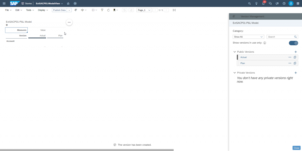
In order to create a new data version we save the story (I named it ‘ExtSACP01-ModelView) then switch from edit mode to view mode.
Here we select the table widget, open the version management panel and create a new version ‘Plan’ with category ‘Planning’
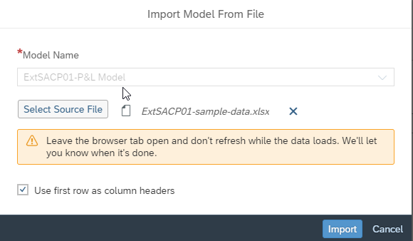
We are ready to import the excel data to the model. Back in the Modeler app, select the Data Management workspace then create a new import job from file. Select the excel file provided.
Once the import job is created, click Set Up Import.
Go to ‘Map to Facts’ step.
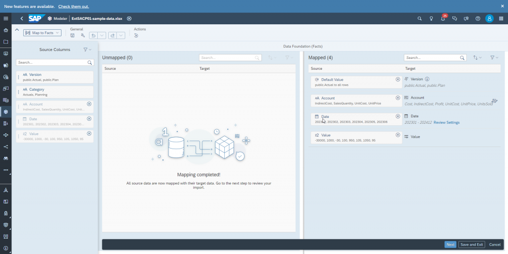
Here we need to delete the default mapping of default.Value = public.Actuals to Version and instead map the csv column ‘Version’
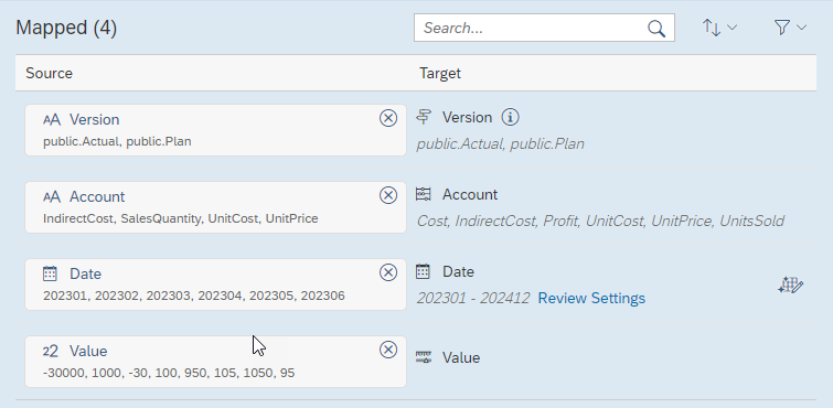
In the next step, ‘Map Properties’, we need to map the csv column ‘Category’ to the Category property of the Version dimension
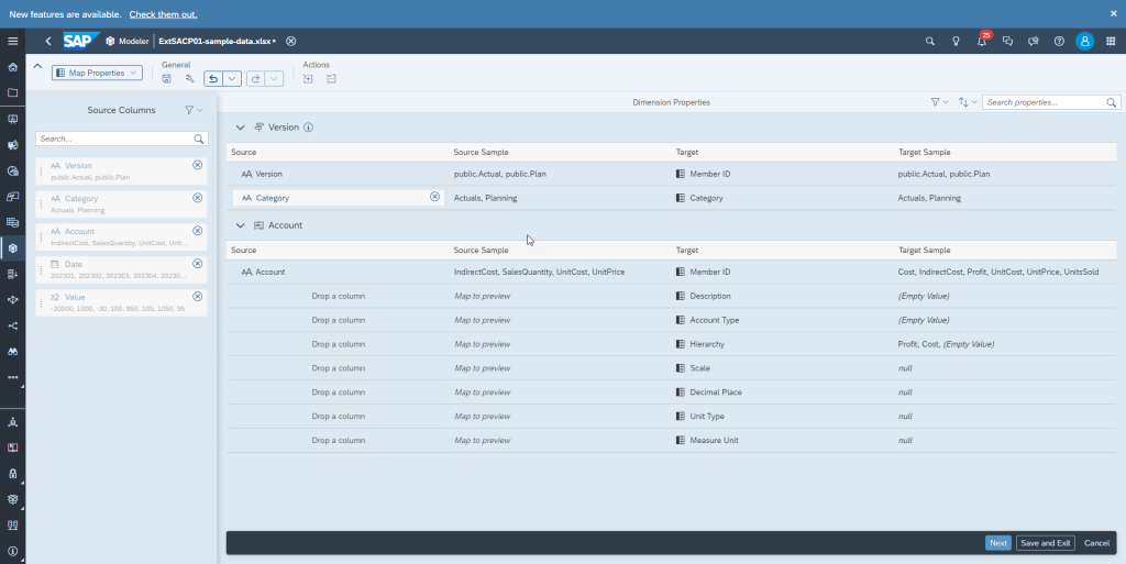
Now we are ready to run the import job which hopefully completes without any problem.
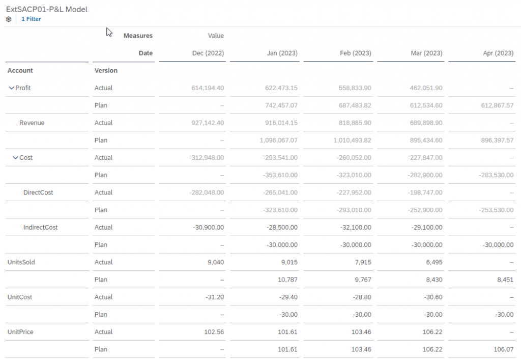
We can check the data inside the P&L model by going back to the story we created earlier.
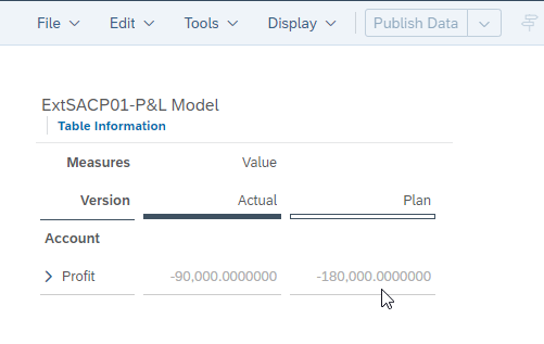
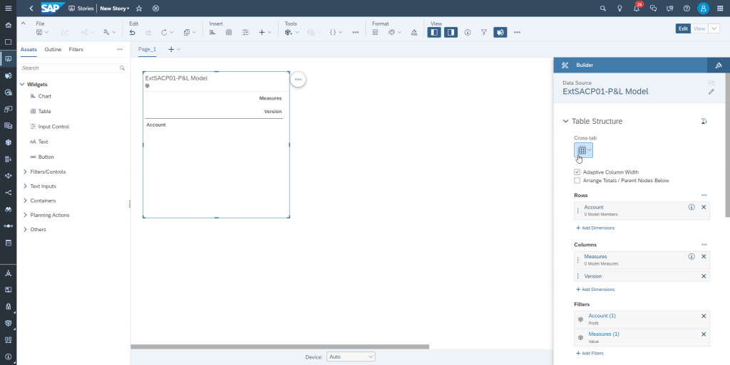
We would like to see a little more detail. Switch to edit mode and open the right side panel. If the panel opens in ‘Styling’ mode, switch to ‘Builder’ mode.
Setup the display to show granular data. Here I have “Account” on rows, “Measure”, “Version” and “Date” on columns.
We would like to allow the planner to enter values for unit price and get estimated values for units sold via ML.
The next step to enable that is to make the data in the Planning model available in DataSphere.
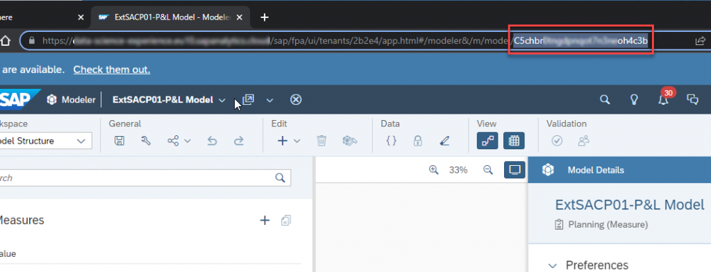
Before leaving SAC, make a note of the model id for the model you created. The model id is the last part of the text in the browser bar when the model is open in the modeler view. We will need it in step 2.3.
2. Expose the data in an SAC model to DataSphere
The SAC model we just created contains ‘fact data’. We want to make this fact data readable from a table – so that we can use it as input for our algorithm.
We are going to achieve this in 3 steps:
- Create an OAuth client in SAC. SAP Datasphere will connect to this client and get data from SAC via this connection
- Create a CDI connection to SAC in Datasphere. This will allow data from SAC to be made visible in Datasphere
- Create a HANA view (in Datasphere) on top of the SAC model fact data
2.1 Create an OAuth client in SAC
this is under System / Administration -> App Integration
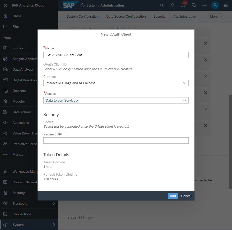
select:
- Purpose: Interactive Usage and API Access
- Access: Data Export Service
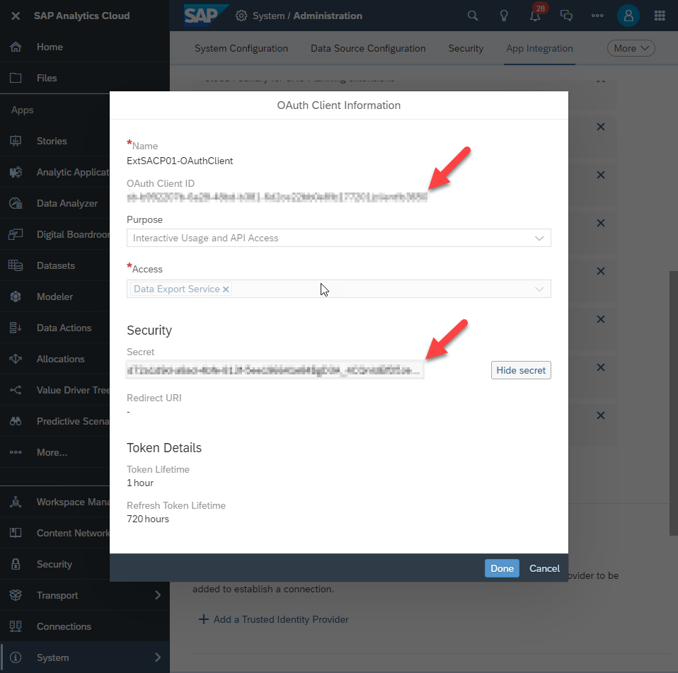
Once the OAuth Client is created, make note of the following pieces of information. We need it in order to create a connection from DataSphere to the OAuth Client in SAC
- SAC system hostname
- OAuth Client ID (generated at creation)
- OAuth Client Secret (generated at creation)
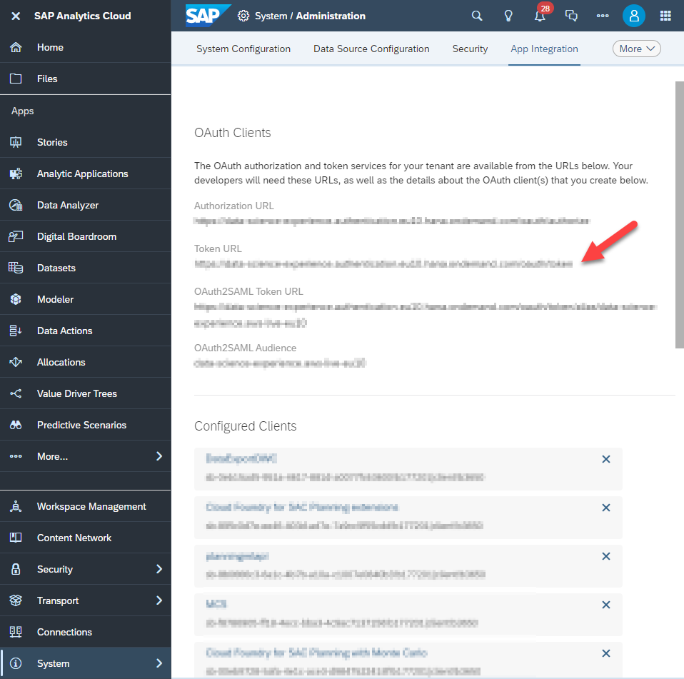
- SAC token URL (displayed at the top of the App Integration page in SAC)
2.2 Create a CDI connection to SAC in Datasphere
In Datasphere connections are defined inside spaces.
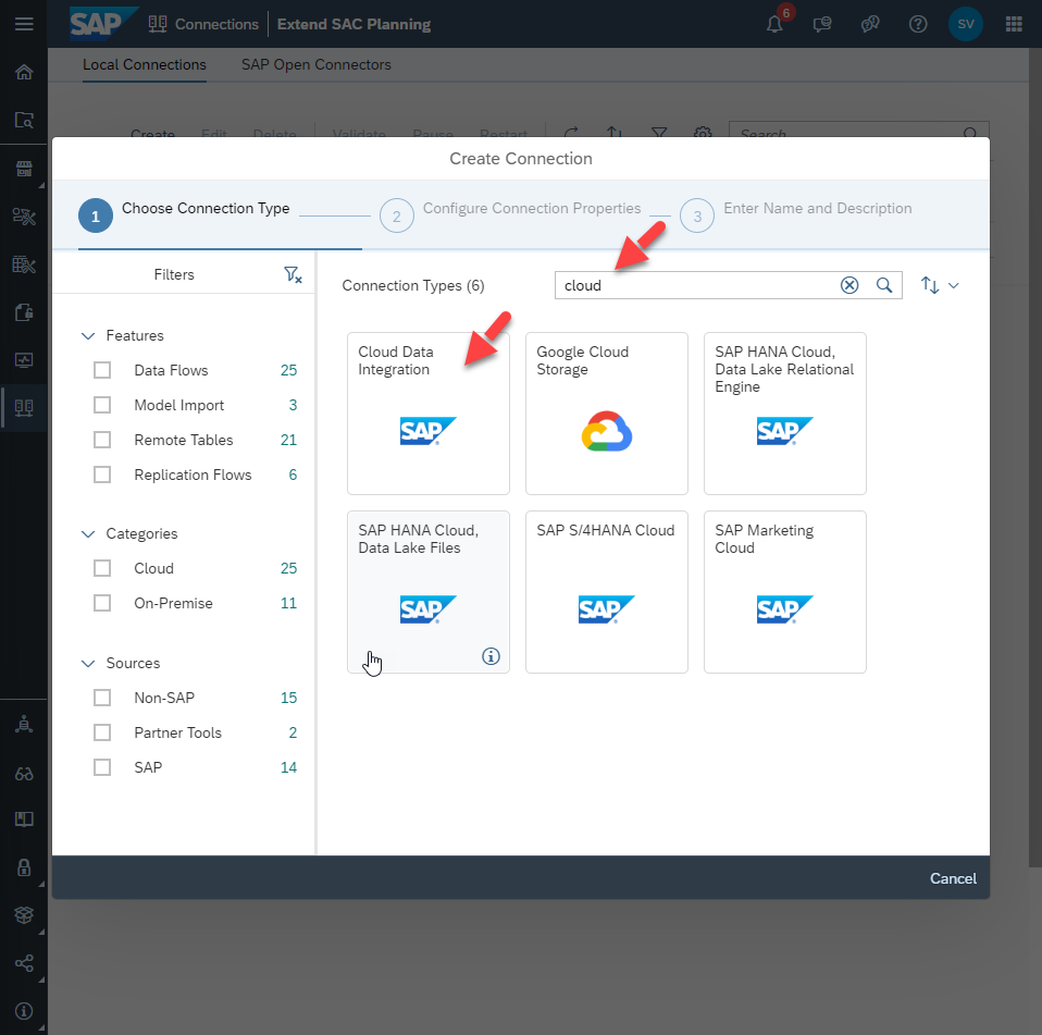
Select your space (in the screenshot it’s ‘Extend SAC Planning’) then go to Connections -> Create
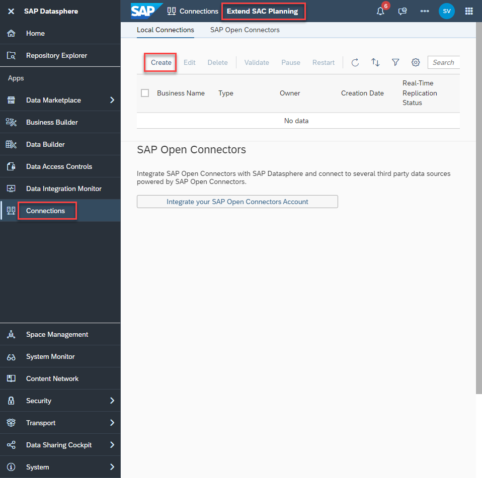
Select a ‘Cloud Data Integration’ connection type:
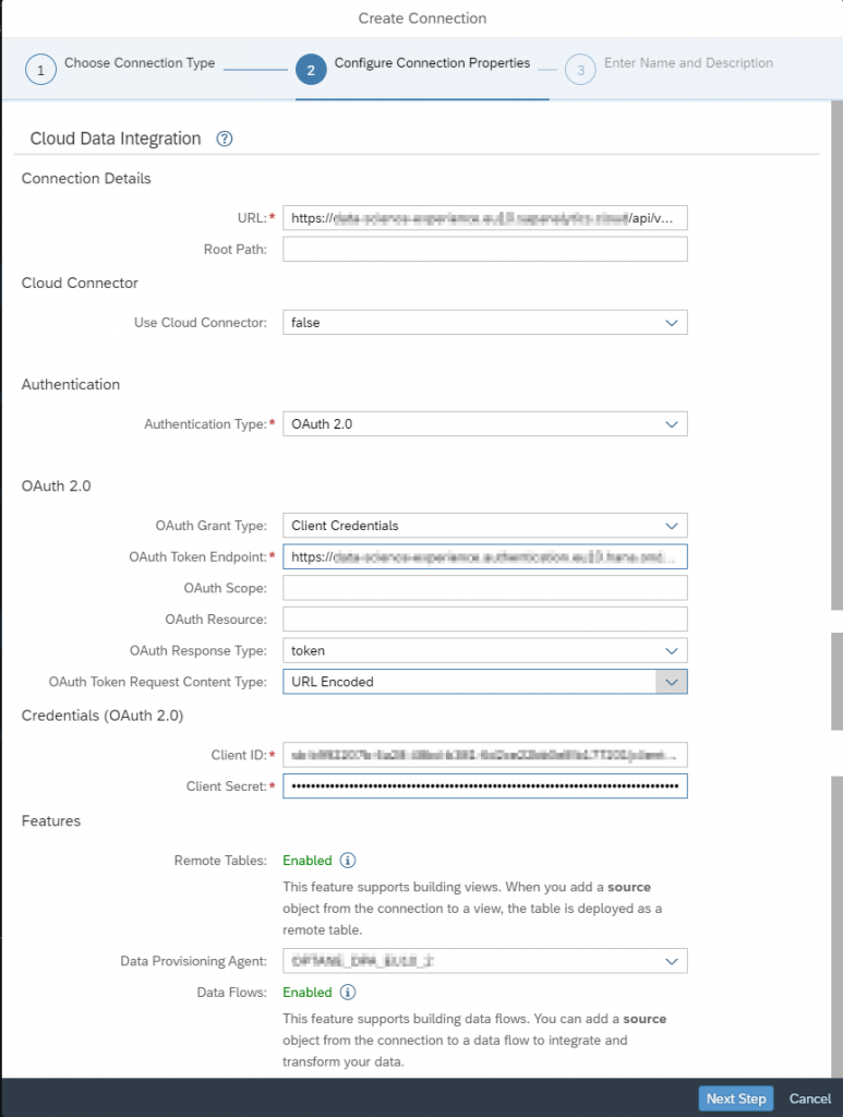
Make the following settings:
- URL: [SAC hostname]/api/v1/dataexport/administration. This the administration service of the Data Export Service of SAC.
- Authentication Type: OAuth 2.0
- OAuth 2.0:
- OAuth Grant Type: “Client Credentials”
- OAuth Token Endpoint: use the SAC token URL we made a note of earlier
- OAuth Response Type: “token”
- OAuth Token Request Content Type: “URL Encoded”
- Credentials (OAuth 2.0):
- Client ID: the OAuth Client ID from the SAC OAuth client (we made a note of it earlier)
- Client Secret: the OAuth Client Secret from the SAC OAuth client (we made a not of it earlier)
- Features:
- Data Provisioning Agent: select a DP Agent to enable Remote Tables
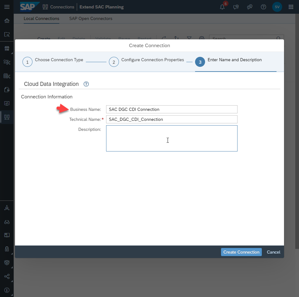
Give a name to the connection.
I used ‘SAC DGC CDI Connection’. DGC is a code that will remind me which particular SAC system this connection goes to.
2.3 Create a HANA view (in Datasphere) on top of the SAC model fact data
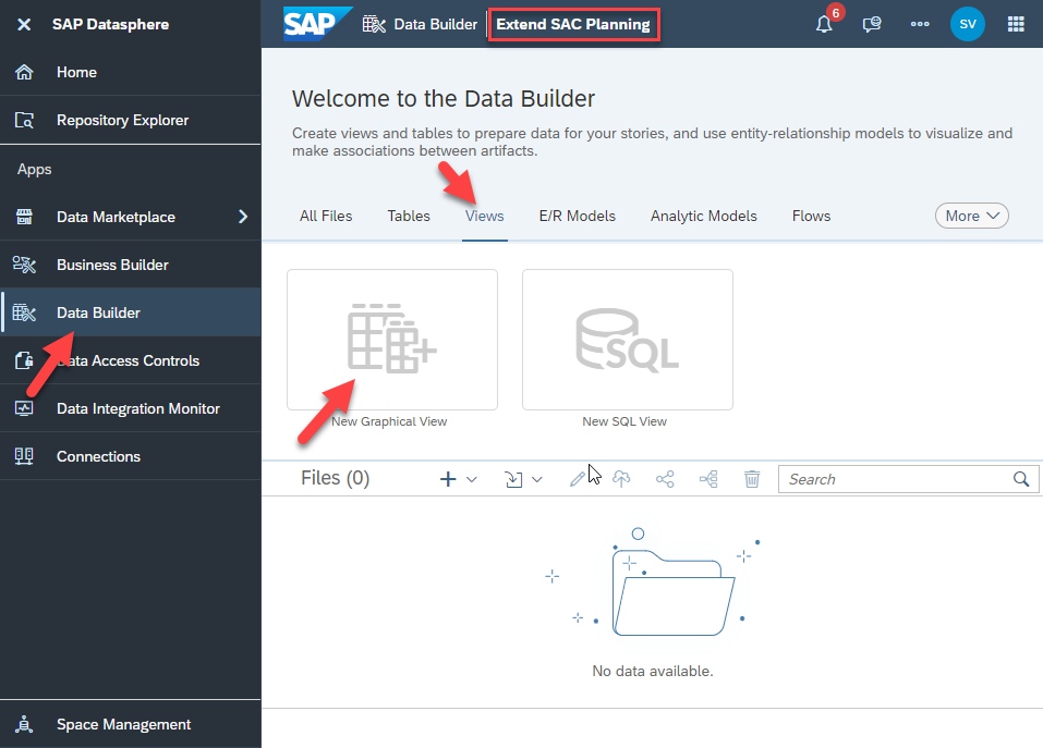
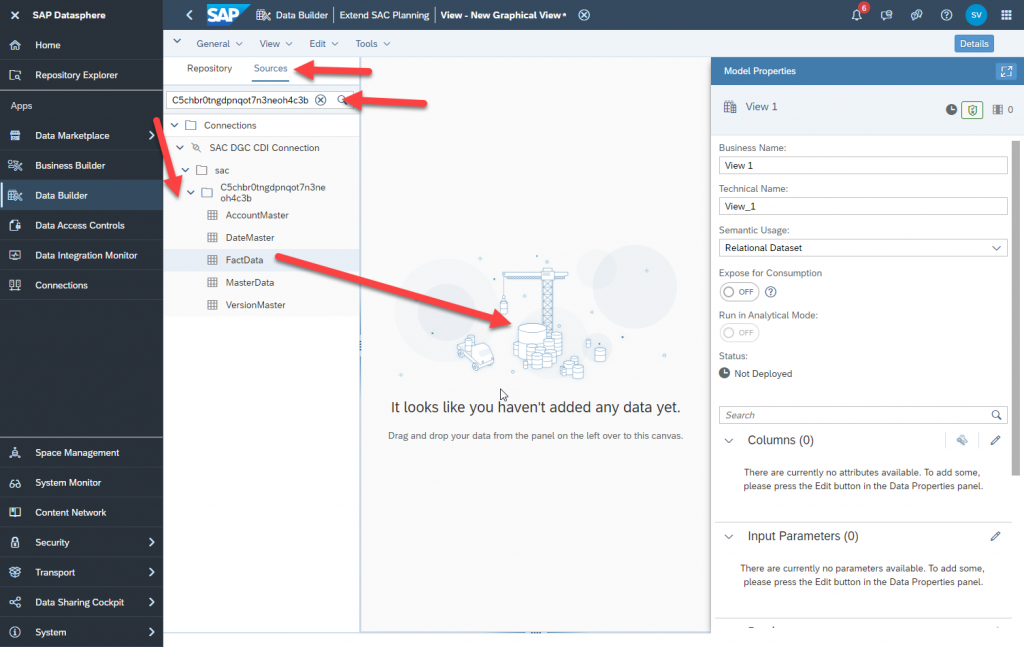
In Datasphere go to ‘Data Builder’. Notice you still need to be in the same ‘space’ where you defined the CDI connection before.
Select ‘New Graphical View’. This will allow us to create the view using the graphical editor.
Go to ‘Sources’ in the left panel. Use the model ID of the SAC Model (the one we made a note of in step 1) in the search box. Drill down to the tables inside the model. Drag ‘FactData’ to the canvas in the middle.
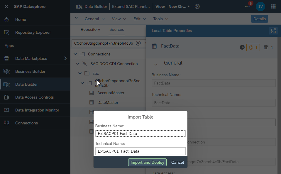
Create a name for the table you are importing then ‘Import and Deploy’.
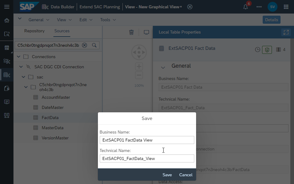
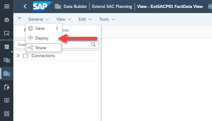
Save the datasphere view. This is in General -> Save.
Make sure the View is exposed for consumption.
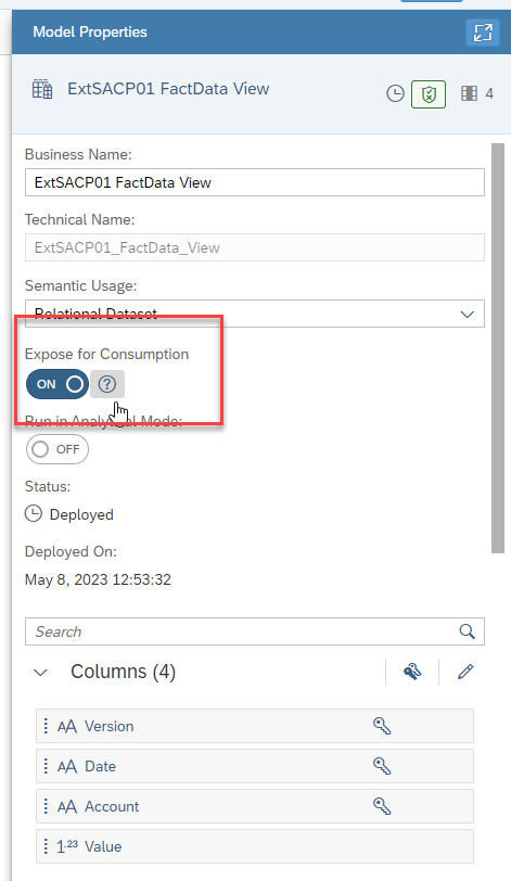
Now the data in the SAC model is accessible from Datasphere. To see the data, drag a column from the View Properties panel to the Data View panel then click view
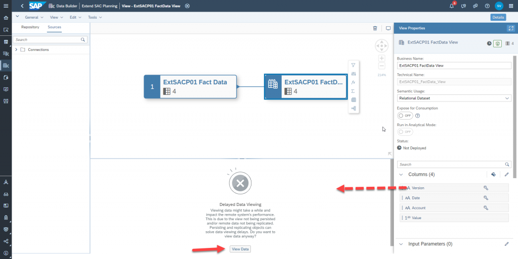
Make sure to deploy the view.
We are almost done. We just need to find the parameters we need in order to connect to the HANA schema inside Datasphere where we just created the view. Once we have that we will be able to access the data in an external API and do any processing we require on it.
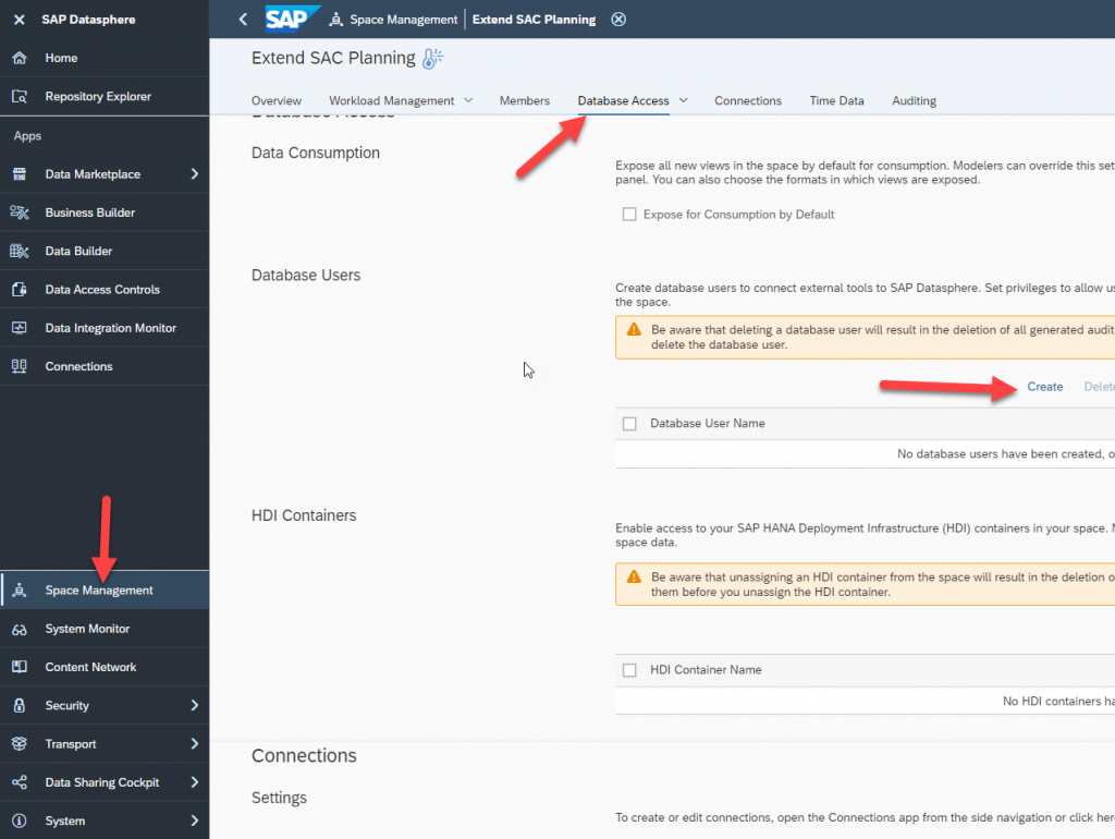
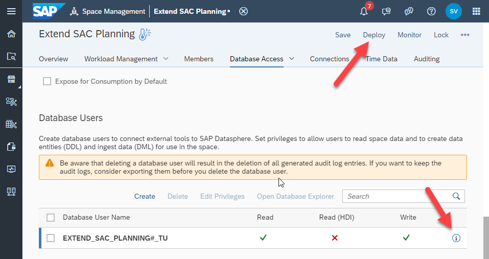
First, we create a Database user in Datasphere. Go to Space Management -> Database Access -> Database Users -> Create
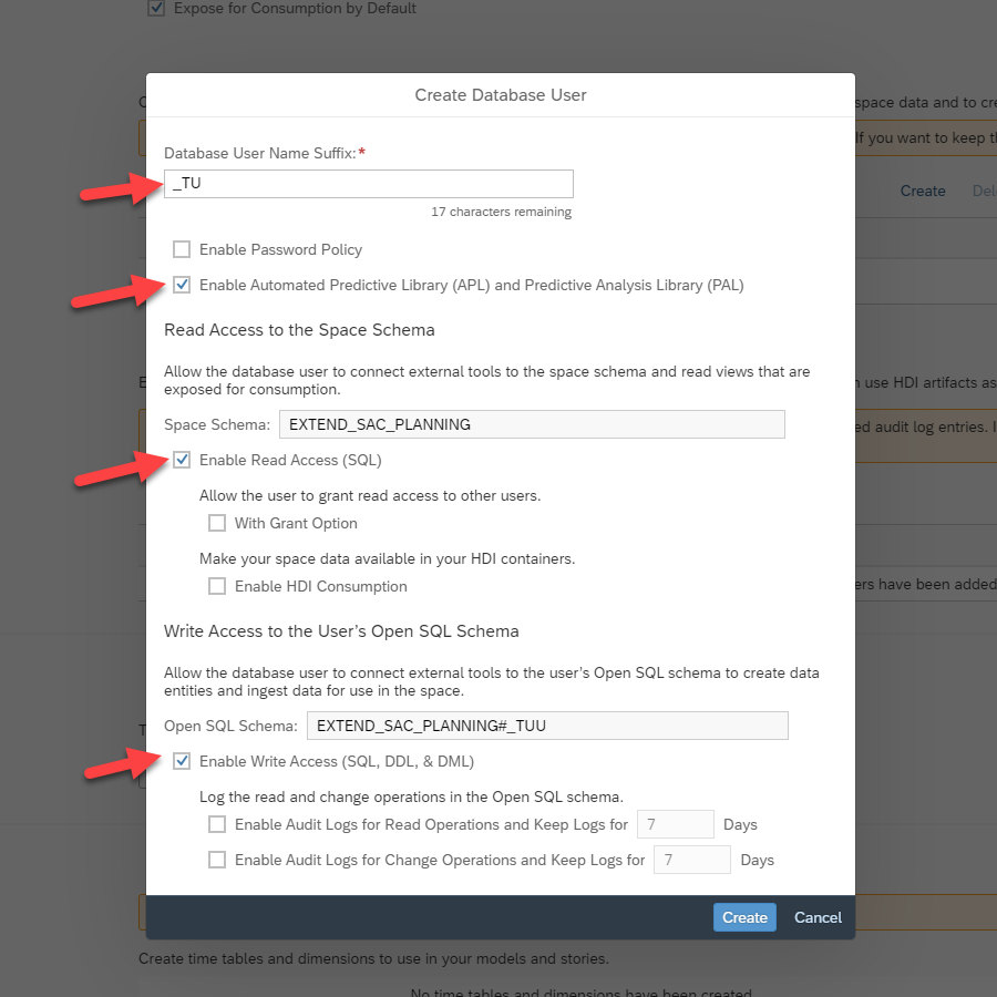
- Set a user name suffix. I chose ‘TU’ meaning ‘technical user’
- Enable read access to the Space Schema
- Enable write access to the User’s Open SQL Schema (this will allow you to write algorithm results here later)
- Enable APL and PAL – these are in-database ML libraries that will be used in the second blog in the series
Deploy the space. Once it’s deployed, open the Database User details view
Make note of:
- Host Name
- Port
- Database User Name
- Password (you will have to click the ‘request new password button’. then the button changes to ‘copy password’)
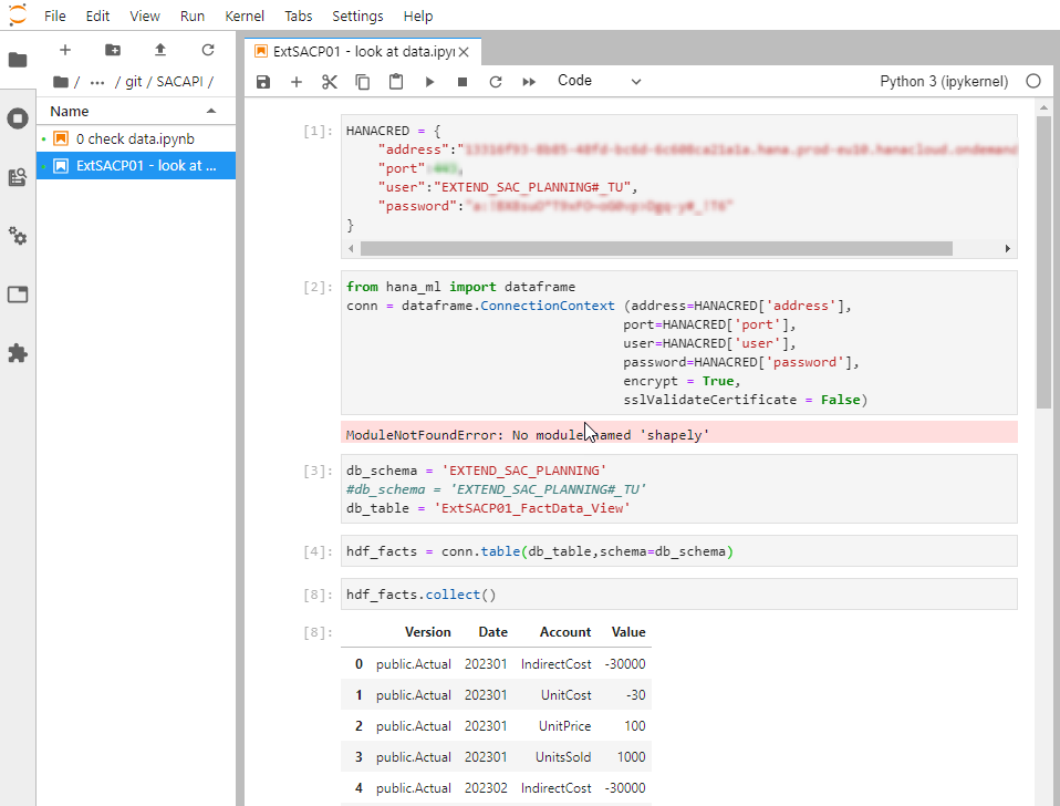
You will use these 4 to connect to the data from an external environment – for example from a Python Jupyter notebook using hana_ml
Also make note of:
- Space Schema – you will find the view on the SAC model fact data here. For me it is EXTEND_SAC_PLANNING
- the name of the view we created earlier – ‘ExtSACP01_FactData_View’
- Open SQL Schema – ‘EXTEND_SAC_PLANNING#_TU’ – this is the Schema that the Database User can write in.
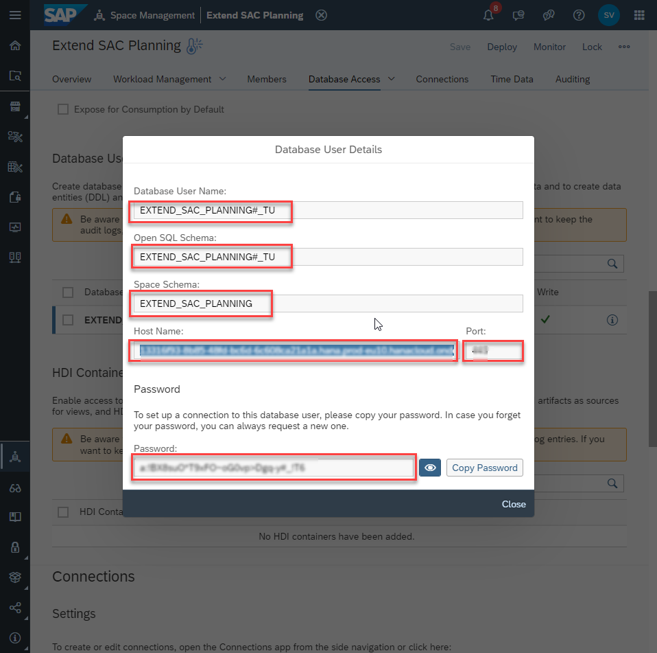
With this information we can access the data from an external algorithm