Introduction
This blog is meant to be a guide to step through the configuration and execution of Demand Driven MRP for S/4HANA On-Premise.
This overview based on S/4HANA 1909 (and, to some degree, for S/4HANA Cloud 1911 and On-Prem 1809).
If you’re preparing for certification or want to strengthen your knowledge in production planning processes, refer to this in-depth SAP S/4HANA Production Planning and Manufacturing Certification Guide. It provides structured learning paths and insights aligned with the key topics discussed in this blog, including Demand Driven MRP and related S/4HANA functionalities.
There is also a DDMRP application that has been designed for SAP IBP (specifically IBP for Inventory but, of course, integrated to other components of IBP to support end-to-end planning solutions).
Although it is possible that some of the applications mentioned in this document will be similar for the set-up of DDMRP in IBP, it is not the intention of this document to discuss those steps.
This guide assumes a starting point of an SAP S/4HANA 1909 system. The user may also find it useful to review the BP script 1Y2i that has been designed to support a test script to support this process as part of SAP Best Practices.
Except for the links to the attached readings, this guide is not meant to provide a detail discussion on the theory of Demand Driven Replenishment.
For this, the user can review the SAP and non-SAP assets listed in the section Initial Reading & Preparation.
This article is meant to provide the user with information of the application set-up and basic understanding of the intentions of these applications for the DDMRP apps designed for SAP S/4HANA.
Initial Reading & Preparation
Amazon: DDMRP Book by Ptak and Smith

General Information Regarding S/4HANA DDMRP Set-Up
General Overview
DDMRP Methodology (Demand Driven Institute)
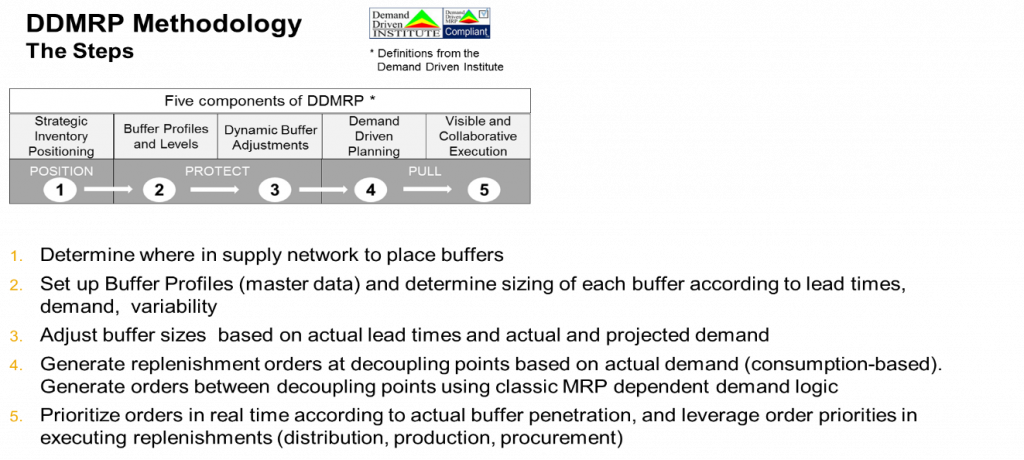
Figure 1.0
Again, the above reading materials can describe in detail these five components of the DDMRP methodology, the important idea here is to recognize each one and to identify the SAP S/4HANA DDMRP app and SAP functionality that is intended to support each component of the methodology.
SAP’s End-to-End Process Flow in S/4HANA
The following represents SAP’s DDMRP end-to-end process flow
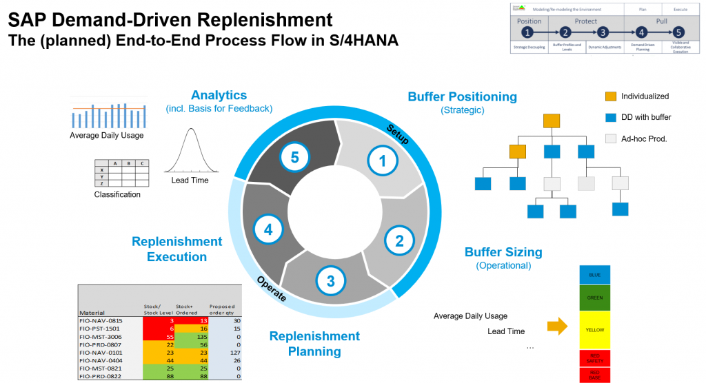
Figure 2.0
The primary objective of DDMRP is to enable material FLOW.
FLOW is key where …
demand is volatile (driven by promotions, innovation, shortening product life cycles, competition…) and there are rigidities in supply (long lead-times, large batches, capacity constraints, …) which result in challenges in service, inventory, speed to market, and ultimately cost.
FLOW is based on these core principles:
Dampening the effect of variation on the supply chain by decoupling lead-times.
This is done through buffers. Identifying where to buffer, and how much to buffer to ensure a) the shortest possible lead-time and b) the most optimum amount of inventory to deal with variation at minimum cost across the chain.
Driving replenishment on actual demand, not forecasts. The best use of our assets is to make what is needed (i.e. what sells). Increasing volatility in demand makes accurate forecasting challenging, even where we have good customer collaboration.
Achieving visibility and prioritization by exposing downstream inventory and demand status to upstream sources to facilitate demand-driven prioritization of supply
SAP S/4HANA Supporting DDMRP apps
The following Fiori apps are intended to support the five DDMRP methodology components from above:
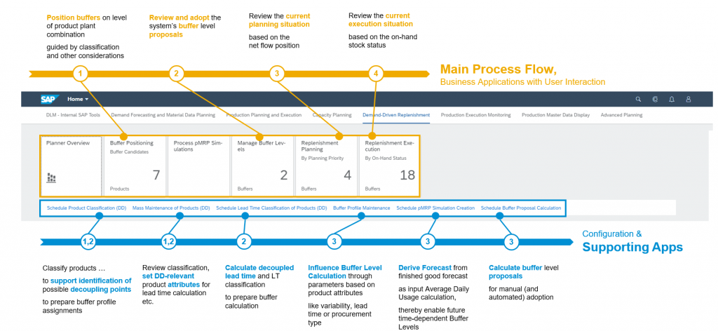
Figure 3.0
Example BOM/Supply Chain used for Demonstration (Simple) – Initial
The following is a simple BOM/Supply Chain example that will be used to demonstrate the DDMRP ideas and SAP DDMRP S/4HANA apps throughout this document.
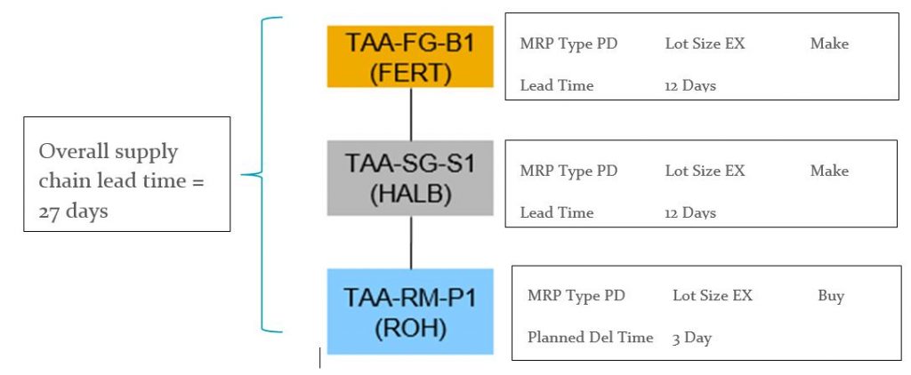
Figure 4.0
Demand Driven Configuration and Set-Up apps
The following are the available apps in S/4HANA that are used to configure and set-up the DDMRP functionality in SAP.
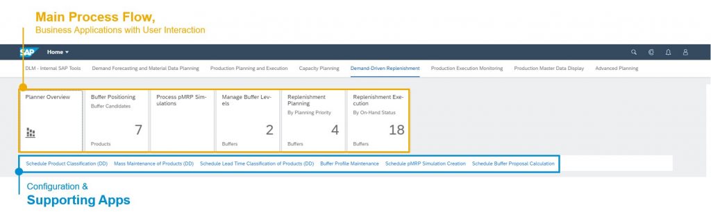
Figure 5.0
The basic design idea for the DDR tile group is …
- … to show the apps with user interaction as tiles, sorted by the process flow
- … to show the other apps (jobs, settings) as links
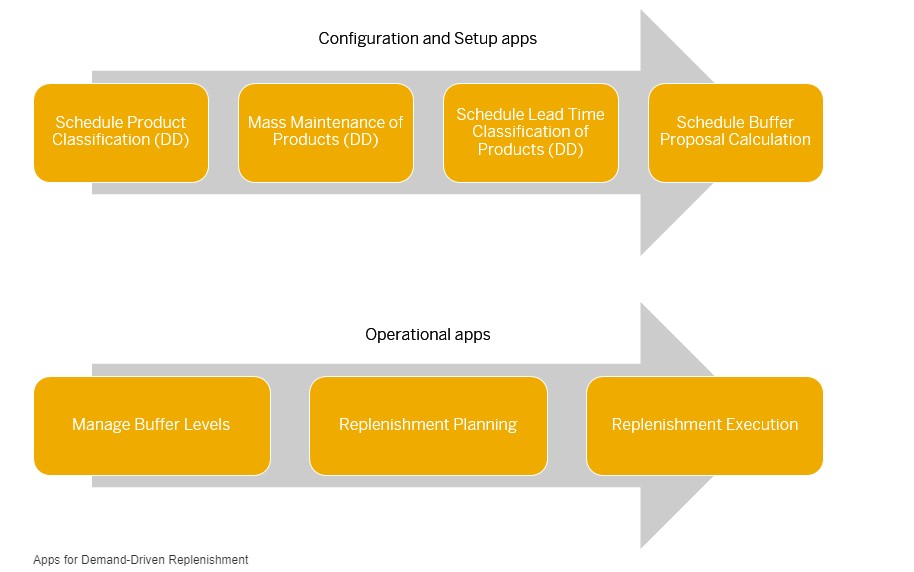
Figure 6.0
Schedule Product Classification (DD) app
General Purpose
Referring to Figure 1.0 and Figure 2.0, this app is most closely aligned with the principle of analyzing all the nodes in the value/supply chain (material networks) that could be considered for decoupling points and buffers candidates in the system.
In practical terms, this app is used to generate and to (later in the Mass Maintenance DD app) to analyze the classifications of inventory value (ABC), variability (XYZ), and BOM usage (PQR).

In its current state, the application only allows for goods issue postings (COGI) to reflect the consumption date for average daily usage (ADU). Material movements documents marked as “consumption data” are not uniquely recognized for this data, rather it is the goods issue movements (cancelled goods issue documents, or course, are not considered).
Practical Use
This is the first app that you’ll use when you start with Demand-Driven Replenishment.
In the parameters within the app, fill in the threshold values for each classification type that are desired to assign to each item considered in the job.
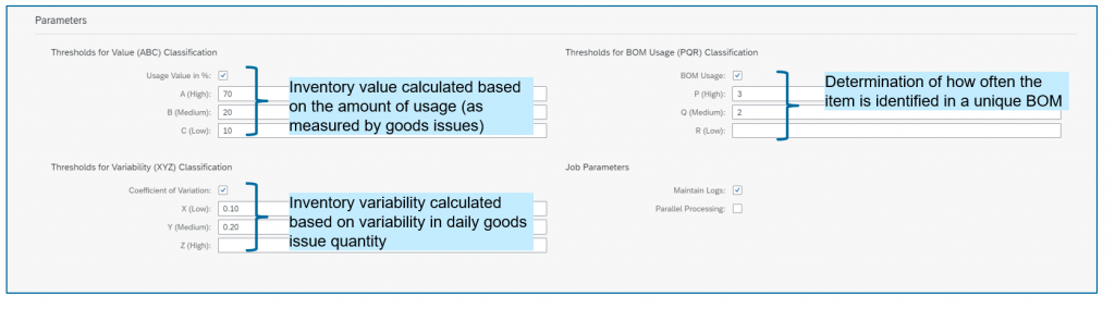
Figure 7.0
Expected Results
The log after the execution of this job might look like the following:
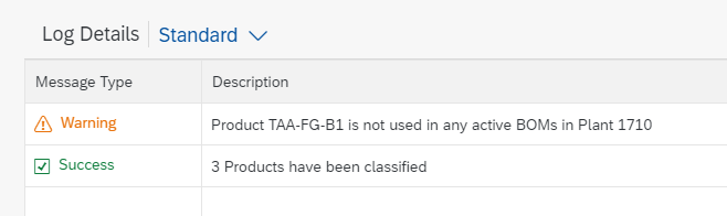
Figure 8.0
This would indicate a successful run. The warning regarding a material not in an active BOM is normal for a finished item that is not consumed within another product structure.
For each item that was successfully processed in this job, the item should now have an assignment to a value classification (high, medium, low), a variability classification (high, medium, low), and a BOM usage indicator (high, medium, low).
These value assignments can be seen in the app Mass Maintenance of Products (DD) as well as in database table PPH_DD_STPR_DETS. Of course, please also review the material consumption table MVER when validating data.
Tips and Tricks Schedule Product Classification (DD) App
If you are setting up a scenario in S/4HANA for the first time, it is important to either post a goods issue at least a day before the current date for the average daily usage to be determined or to run the job at the end of the calendar day for the average daily usage statistic to be calculated.
This is important because the job will provide a hard error (for the material in question) if an ADU statistic cannot be generated.
Product classifications can change seasonally or based on increase or decrease in demand over time. SAP recommends that you periodically re-classify your products to ensure that the right products are considered relevant for Demand-Driven Replenishment.
Mass Maintenance of Products (DD)
General Purpose
This is the second app that you’ll use when you start with Demand-Driven Replenishment.
Referring to Figure 1.0 and Figure 2.0, this app is most closely aligned with the action of systematically setting the buffers within the supply chain(s) of your evaluation.
Practically, this is done by setting the MRP type, Lot Sizing Procedure, and Horizon to those that match you DDMRP strategy.
After the products have been classified or re-classified, you can view the results of the classifications in this app, and based on the results, select products that are relevant to Demand-Driven Replenishment.
With the mass change feature you will change the master data records for several products simultaneously.
The products are classified based on goods issue value (ABC Classification), usage across BOMs (PQR Classification) and variation in actual demand (XYZ Classification) using the Schedule Product Classification (DD) app in the previous step.
Typically, products with the highest goods issue value (type A), longest lead times (type G), highest BOM usage (type P) and highest variability (type Z) are relevant for Demand-Driven Replenishment. It is a business decision to select DD-relevant products, as the next tier of classifications, B, F, Q and Y, can also be considered if desired.
Fiori App Library Entree: Mass Maintenance of Products (DD) App

Practical Use
After After filtering the app for our products, the output could look like this initially:
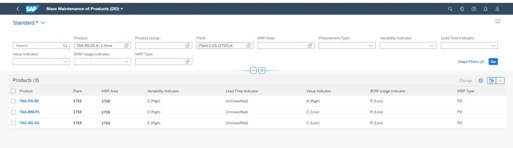
Figure 9.0
If we review Figure 2.0 again, we are reminded that this app primarily supports the idea of maintaining the MRP type (D1) such that we have determined the buffer(s) in our supply chain.
After classifying each material in the previous app, we now have additional data (ABC, XYZ, PQR analysis) that could be used to support this type of decision (often this determination is already natively known by each customer by much greater analysis).
The User selects products that are relevant for Demand-Driven Replenishment based on the results of their product classification
At any rate, for our example, let’s assume we know that we would like to set a buffer for the material TAA-SG-S1. We can use this app to change the MRP Type (to D1), the Lot Size Procedure (to H1) and the Horizon for the Past (to 15 days)
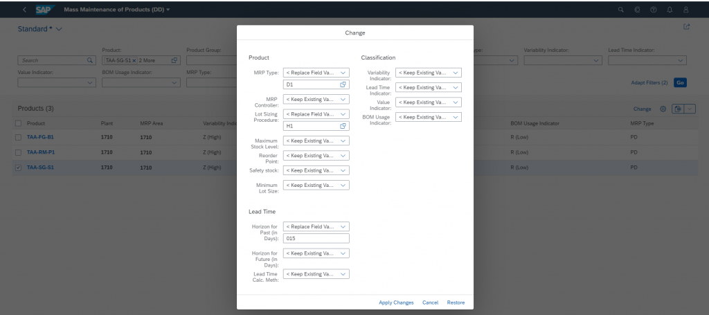
Figure 10.0
Expected Results
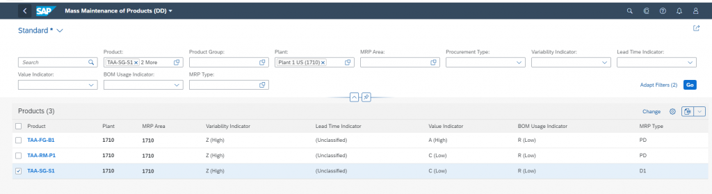
Figure 11.0
Schedule Lead Time classification of Products (DD) app
General Purpose
Referring to Figure 1.0 and Figure 2.0, this app is most closely aligned with the action of setting the buffers within the supply chain(s) of your evaluation by systematically calculating the lead time classification and determining the decoupled lead times assigned to the previously determined supply chain buffers.

Fiori App LibrarySchedule Lead Time Classification of Products (DD) App
Practical Use
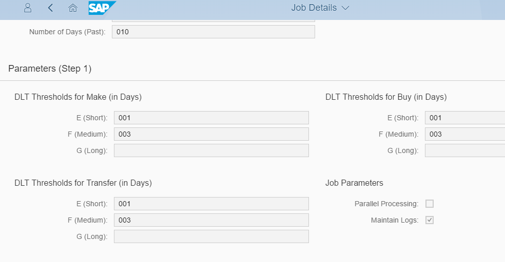
Figure 12.0
Expected Results
Of course, the expectation here is that a lead time indicator is set (as shown in Figure 13.0).
This along with the variability indicator that was set in the Schedule Product Classification (DD) app will be used later to help determine the variability and lead time factors.
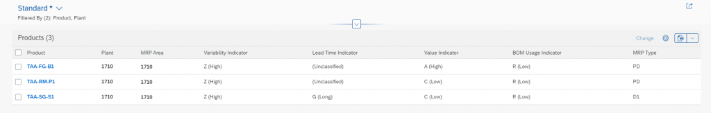
Figure 13.0
Tips and Tricks
This job will only add lead time indicator values to those items that you had previously marked as being Demand Driven MRP relevant through the setting of the MRP Type.
Example BOM/Supply Chain Used for Demonstration (Simple) – Updated
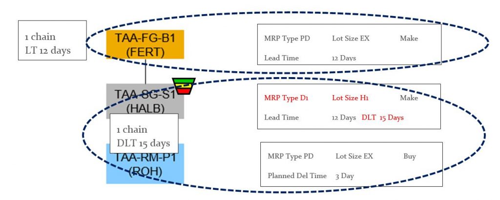
Figure 14.0
Schedule Buffer Proposal Calculation App
General Purpose

Referring to Figure 1.0 and Figure 2.0, this app is aligned with the action of systematically calculating the buffer proposal(s) for the identified supply chain buffers /products, based on their average daily usage, decoupled lead time, buffer profiles and several other factors.
Fiori App Library Entree:Schedule Buffer Proposal Calculation App
Practical Use
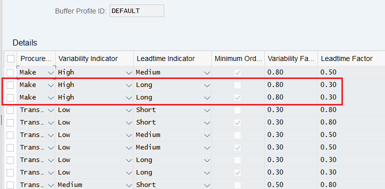
Figure 15.0 (Buffer Profile: Transaction SM34, View Cluster = PPH_DD_PROFILE_ASG_VC)
Calculation Chart used to determine each buffer quantity:
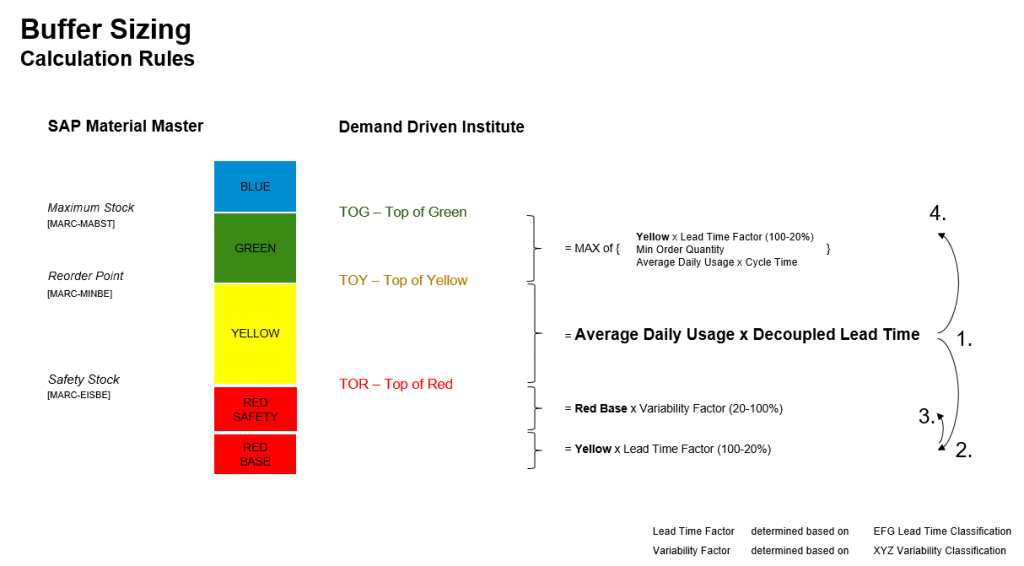
Figure 16.0
The buffers are primarily calculated based on the ADU of the material’s issues, the decoupled lead time, and the variability and lead time factors.
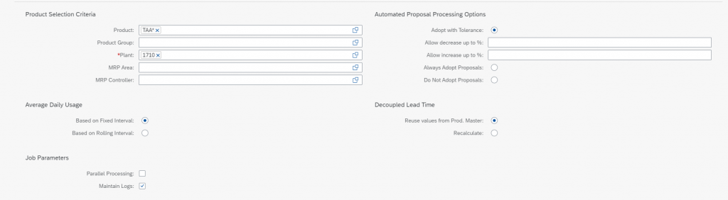
Figure 17.0
Tips and Tricks
Use table PPH_DD_STPR_HDR to confirm DD parameters and factors
Use table PPH_DD_STPR_DETS to confirm material’s ADU
Use table PPH_DD_STPR_COMP to confirm BOM component’s lead time
Through adoption, the new buffer levels are written into DB table PPH_DD_STK
The tables PPH_DD_STPR… contain the buffer level proposal
BUSINESS APPLICATIONS WITH USER INTERACTION APPS
Referring to Figure 5.0 DDR apps with user interaction are shown as tiles, sorted by the process flow
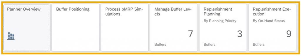
Figure 18.0
Planner Overview app
General Purpose
Fiori App Library Entree: Planner Overview APP
The Planner Overview informs the user with a set of cards about the most important information and tasks in the actual planning situation.
The planner can view, filter, and react promptly to DDR planning situation.
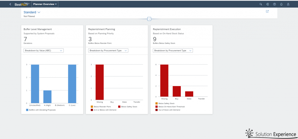
Figure 19.0
Practical Use
The planner can see the key figures, which are also visible on the Fiori Launchpad tiles:
- Buffer proposals to be review
- Buffers to be planned
- Low on-hand buffer fill level to be managed
The key figures can be broken down by different dimensions:
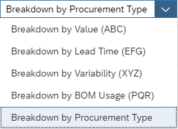
By click on a stacked bar, the user navigates into the respective work list.
Buffer positioing (DD) App
General Purpose
With this app the you can identify products to be buffered by analyzing the upstream and downstream of the products in the supply chain.

Fiori App Library Entree: Buffer Positioning (DD) App
The following items should be considered as preparation of the Buffer Positioning:
- Is the product a candidate for consumption-based planning?
- -> Look at the ABC-XYZ-matrix (value & variability)
- Is the product used in many BOMs?
-> Evaluate the BOM usage - How reliable is the source?
- How long is my customer willing to wait?
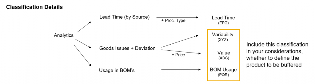
Figure 20.0
In addtition to the classifications you can filter candidates for decoupling
by Use-Case-specific
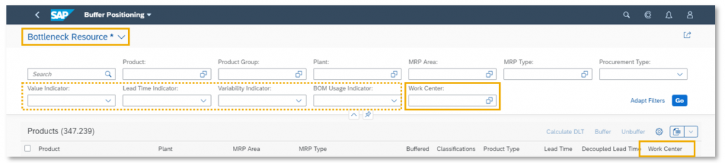
Figure 21.0
Bottleneck Protection (1808)
Objective: Components which are consumed at a bottleneck work center should be available
Procedure
- Select by bottleneck work centers
- Derive buffer candidates (component products) via production version
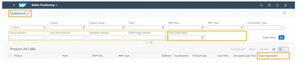
Figure 22.0
Outbound Protection (1805)
Objective: Ensure to meet response time expected by the customer
Procedure
- Select sold products by sales organization
- Check the calculated decoupled lead time
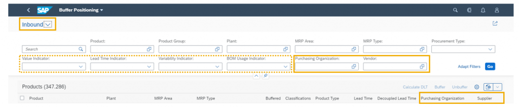
Figure 23.0
Inbound Protection
Objective:
Stabilize the material flow within my company through protection against supply variability
Procedure
- Select by purchase organization & supplier
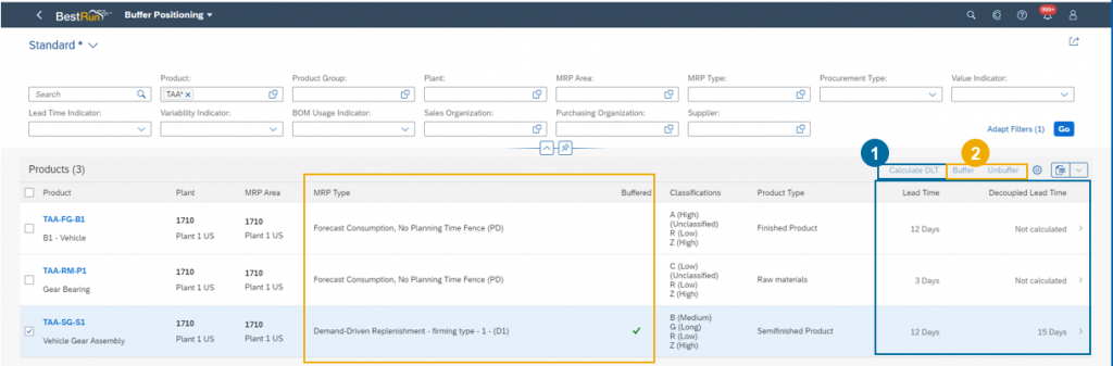
Figure 24.0
In the Worklist you can review the selected candidates, identify and define the decoupling points.
Procedure:
In step 1 you can re-calculate On-demand certain key attributes and in step 2 execute the action to buffer by assigning MRP Type = D1 (Demand-Driven) to the candidates.
You can drill down to analyze a potential decoupling point in Detail.
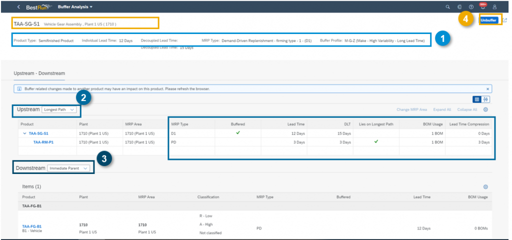
Figure 25.0
You can review key attributes (1) like classification, DLT, Buffer Profile.
Review the Upstream (2) incl. BOM Usage, achievable Lead Time Compression …
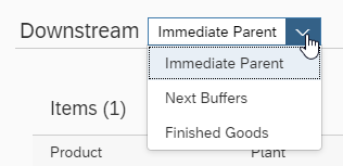
Review the Downstream (3) which following buffers could be reduced if TAA-SG-S1 was buffered which finished goods would benefit
The Planner can take the action to (un-)buffer (4) a candidate here or drill down into further details of the supply chain / multi-level BOM…
The User can also toggle between a tree table and network graphics

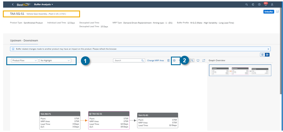
Figure 26.0
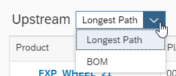
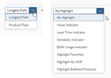
The Network Graphic supports Buffer Analysis by (1)…
- setting scope (longest path vs. full flow)
- highlight by selected attributes
- (partial) collapse and expand of network
- navigation into next product(s)
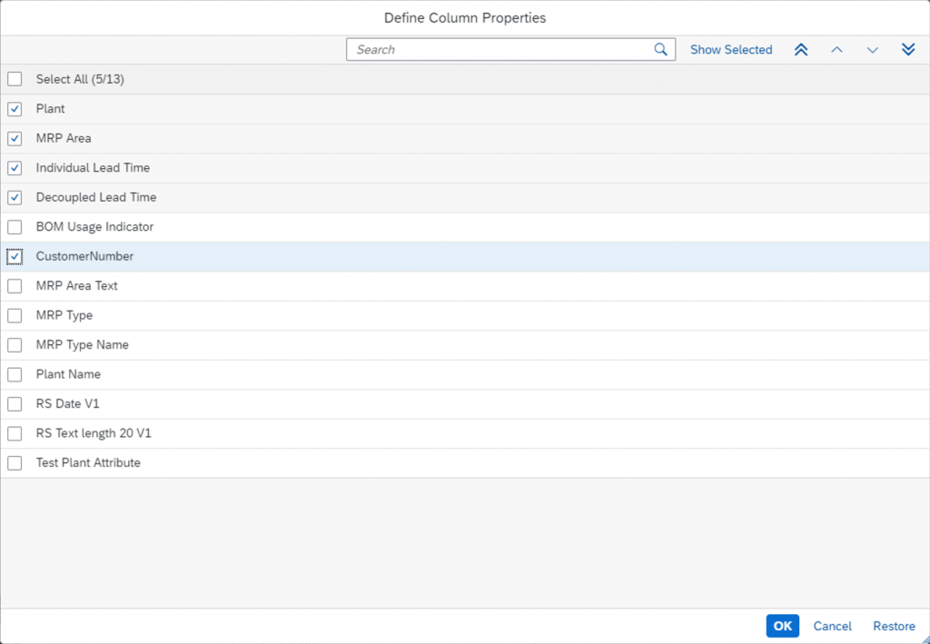
In Define Column Properties (2) it is possible to add Product-Master-specific custom fields to the UI
The “Administrator” is thedefault key-user, it has permissions to:
- Create Custom Field
- Assign custom field to application
- Add field in UI with UI adaptation
Manage buffer levels app
General Purpose
Referring to Figure 1.0 and Figure 2.0, this app is aligned with the review for adoption the previously calculated buffer proposals.

Fiori App Library Entree:Manage Buffer Level App
Practical Use
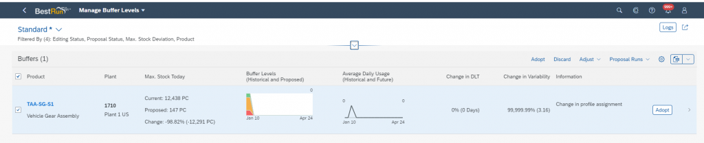
Figure 28.0
If it is important to review the details that are behind the new proposal(s), the user can click on the right arrow to review the analytics and object pages of the relevant information.
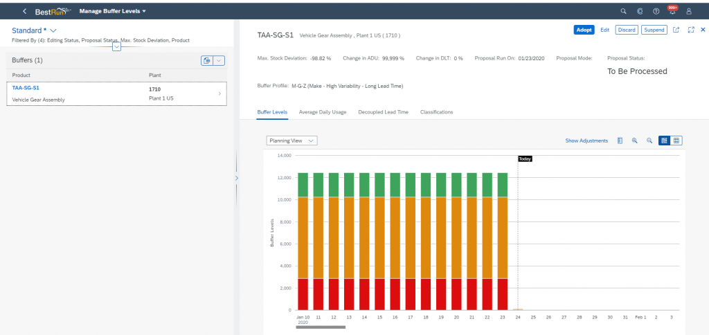
Figure 29.0
Tips and Tricks
Use table PPH_DD_STK can be used to review saved buffer values
Proposals are stored in DB tables PPH_DD_STPR
Replenishment Planning app
General Purpose
Referring to Figure 1.0 and Figure 2.0, this app is used to review the current planning situation based on the net flow Position.
Fiori App Library Entree:Monitor Demand Driven Replenishmen
Practical Use
The main idea here would be to prioritize the planning of supply orders by evaluating the net flow position of supply elements in relation to buffer status.
This is considered based on the following calculation:
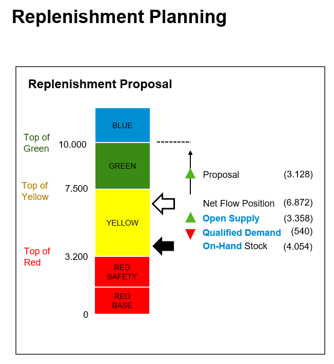
Figure 30.0
Net flow position = On-Hand Inventory + Open Supply – Qualified Executable Order Demand
Where On-Hand Inventory is equal to the qualified available stocks, Open Supply is equal to the available order proposals (production orders, planned orders, stock transfer orders, purchase requisitions, purchase orders) and where Qualified Executable Demand is equal to firm/executable demand that is backordered, due today, or is identified as a qualified “spike” in the future.
Qualified Spikes
The purpose of considering qualified spikes in the net flow position is to manage the buffer in a way that protects it from irregularities in future consumptions that may not be considered based on the current variability and lead time factors that were used to construct the existing Buffers.
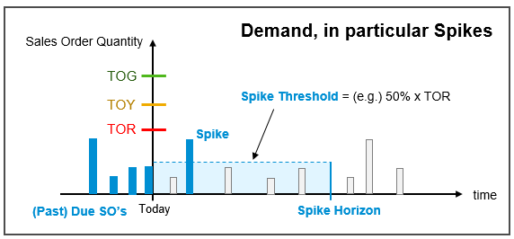
Figure 31.0
The spike is identified by reviewing all qualified demands in the spike horizon and has exceeded the spike threshold previously determined based on the buffer profile settings.
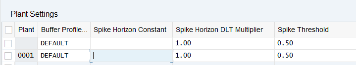
Figure 32.0
These spike parameters are determined based off the following inputs and calculations:
Spike Horizon Constant (SHC)
A constant, usually measured in days, which helps calculate the Order Spike Horizon when summed with the product of the Spike Horizon DLT Multiplier (SHM) and the Decoupled Lead Time (DLT).
Order Spike Horizon = (SHM x DLT) + SHC
Spike Horizon DLT Multiplier (SHM)
A multiplicative factor that when multiplied with the Decoupled Lead Time (DLT) and summed with a Spike Horizon Constant (SHC) helps calculate the order spike horizon, which helps identify order spikes.
Order Spike Horizon = (SHM x DLT) + SHC
Spike Threshold Factor
A selected quantity that in combination with the Order Spike Horizon qualifies an order spike
Once the net flow position is calculated, it can be reviewed against the planning priorities in the Replenishment Planning app and reviewed against the expected proposed quantities needed to bring the buffer for the plant material combination back to target. These Proposed Quantities would normally be generated in the next MRP (MRP Live) planning run.
Demand-Driven Planning, fully embedded in the context of the MRP Run.
Buffered products are defined through the assigned MRP type = D1 (MRP Procedure = C). They participate in the MRP Run (both classic MRP and MRP Live)
Their net requirement logic is demand-driven, defined through this MRP Type / MRP Procedure
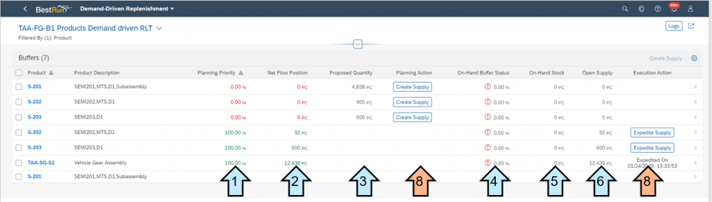
Figure 33.0
- Planning Priority: Net Flow Position/ Max Stock
- Net Flow Position: Current flow position
- Proposed Quantity: Amount of quantity needed to bring inventory back to target. This is also the amount of planned order quantity that would be expected to be generated during the next MRP run. If NFP is below reorder point, i.e. status is yellow or worse
- On-Hand Buffer Status; Amount of on-hand stock percentage of safety
- On-Hand Stock: Amount of on-had stock
- Open Supply: Amount of make/buy/transfer orders in the system for this material
- Quick action to create supply or expedite supply
Net flow position = On-Hand Inventory + Open Supply – Qualified Executable Order Demand
You can navigate into object page for detailed planning by clicking on a line
On a Object Page you will see the comprehensive Buffer Context for a consistent DDR Planning (in the Tree)
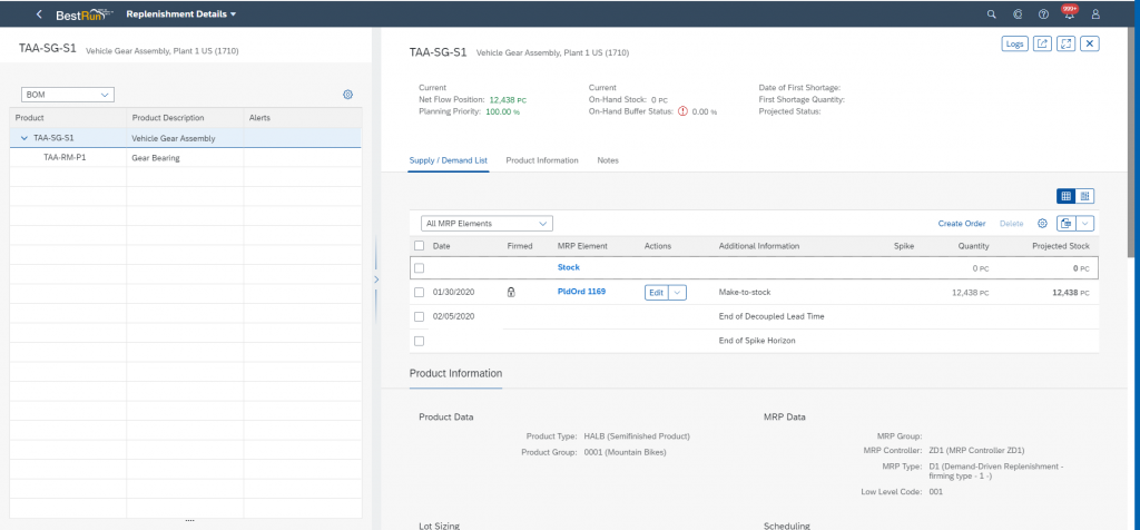
Figure 34.0
The object page will provide information like Multi-level BOM for the buffered product, you can directly navigate into details of components’ supply & demand lists and you can Interactively change orders.
Replenishment execution app
General Purpose
Referring to Figure 1.0 and Figure 2.0, this app is used to review the execution situation based on the on-hand stock Status.
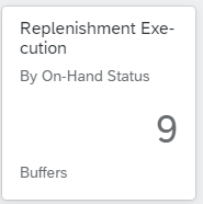
Fiori App Library Entree: Monitor Demand Driven Replenishment
Practical Use
The main idea here would be to expedite orders through prioritization by evaluating the order penetration of the safety (RED) Buffer.
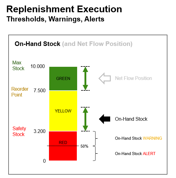
Figure 35.0
Usually the On-Hand Stock oscillates between
- <Safety Stock> and
- <Safety Stock + Green Zone> If it falls below 50% of the safety stock, the system raises an ALERT that the actual material flow is severely endangered.
- Note: The Net Flow Position might still look OK. But inbound supply is of little or no help if there is no actual stock at hand in the shop floor
- If it falls below the safety stock level, the system raises a WARNING that the actual material flow is endangered.
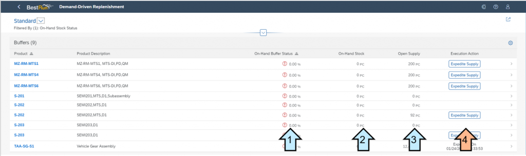
Figure 36.0
- On-Hand Buffer Status; Amount of on-hand stock percentage of safety
- On-Hand Stock: Amount of on-hand stock
- Open Supply: Amount of make/buy/transfer orders in the system for this material
- Quick action to Expedite Supply
Also, in this app you can navigate into object page by clicking on a line
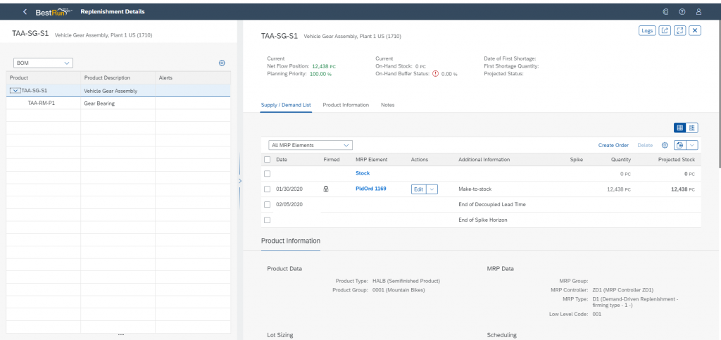
Figure 37.0
The Object page supports all the features which are already highlight in section “DD Planning


