Introduction
The detection of anomalies from a given time-series is usually not an easy task. The natural association with time brings many unique features to time-series that regular 1D datasets, like time-dependency(via lagging), trend, seasonality, holiday effects, etc. Because of this, traditional statististical tests or clustering-based methods for anomaly/outlier usually will fail for time-series data, because the time information of time-series is ignored by their design of nature. In other words, the applicability of statistical tests at least requires time-series data values to be time-independent, yet this is often not guaranteed. However, with appropriated modeling, a roughly time-indepdent time-series can often be extracted/transformed from the original time-series of interest, in which case statistical tests becomes applicable. One such technique, also the main interest of this blog post, is seasonal decomposition.
Basically, seasonal decomposition decomposes a given time-series into three components: trend, seasonal and random, where:
- the seasonl component contains patterns that appears repeatedly between regular time-intervals(i.e. periods)
- the trend component depicts the global shape of the time-series by smoothing/averaging out local variations/seasonal patterns
- the random component contains information that cannot be explained by seasonal and trend components(values assumed to be random, indicating time-independent)
The relation between the original time-series data and its decomposed components in seasonal decomposition can either be additive or multiplicative. To be formal, we let X be the given time-series, and S/T/R be its seasonal/trend/random component respectively, then
- multiplicative decomposition: X = S * T * R
- additive decomposition: X = S + T + R
It should be emphasized that, for multiplicative decomposition, values in the random compnent are usually centered around 1, where the value of 1 means that the original time-series can be perfectly explained by the multiplication of its trend and seasonal components. In contrast, for additive decomposition, values in the random compoent are usually centered around 0, where the value of 0 indicates that the given time-series can be perfectly explained by the addition of its trend and and seasonal components.
In this blog post, we focus on anomaly detection for time-series that can largely be modeled by seasonal decomposition. In such case, anomalous points are marked by values with irregularly large devivations in the random component, which correspond to unexplained large variations beyond trend and seasonality.
The Use Case : Anomaly Detection for AirPassengers Data
In the following context we show a detailed use case for anomaly detection of time-series using tseasonal decomposition, and all source code will use use Python machine learning client for SAP HANA Predictive Analsysi Library(PAL). The dataset we use is the renowned AirPassengers dataset firstly introduced in a textbook for time-series analysis written by Box and Jenkins.
Connection to SAP HANA
Assuming the dataset is stored in SAP HANA as a table with name ‘AIR_PASSENGERS_TBL’. Then, we can fetch the data via a connection to the database.
import hana_ml
from hana_ml.dataframe import ConnectionContext
cc = ConnectionContext('xx.xxx.xxx.xx', 30x15, 'XXX', 'Xxxxxxxx')#account info hidden away
ap_tbl_name = 'AIR_PASSENGERS_TBL'
ap_df = cc.table(ap_tbl_name)
Dataset Description and Pre-processing
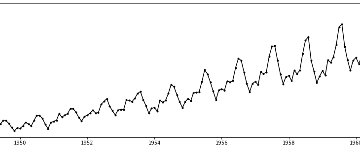
The AirPassengers dataset is a monthly record of total airline passengers between 1949 and 1960, illustrated as follows:
ap_data = ap_df.collect()
ap_data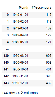
The dataset contains two columns : the first column is the month info(represented by the first day of each month), and the second column is the number of passengers(in thousands). Now we draw the run-sequence plot of this dataset for better inspecting its shape and details.
import matplotlib.pyplot as plt
plt.plot(pd.to_datetime(ap_data['Month']), ap_data['#Passengers'])
plt.show()
Before applying any time-series analysis method to this dataset, we add an ID column of integer type. We do so because an ID column of integer type is a must for most time-series algorithms in hana_ml, inclusive of seasonal decomposition. Besides, the added integer ID column must represent the order of values for the time-series data, so generated IDs must follow the order of timestamps of the time-series. We can generate such an ID column using the add_id() function of hana_ml.DataFrame as follows:
ap_df_wid = ap_df.cast('Month', 'DATE').add_id(id_col='ID', ref_col='Month')Now we may check whether everything is okay after the new integer ID column has been added.
ap_df_wid.collect()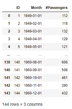
Multiplicative Decomposition
Observing from its run-sequence plot, the AirPassengers dataset clearly has trend and seasonality: the number of airline passengers keep growing year-by-year, forming an upward trend; within each year there is a clear seasonal pattern – high in year middle and low in year start/end. Note that the seasonal variations become larger as the number of passengers increases, which is a clear evidence for multiplicative seasonality. Seasonal decompostion is implemented by the function seasonal_decompose() in hana_ml, we can import the function and then apply it to the original time-series to verify our justification on the type of decomposition.
from hana_ml.algorithms.pal.tsa.seasonal_decompose import seasonal_decompose
stat, decomposed = seasonal_decompose(data = ap_df_wid,
                                      key = 'ID',
                                      endog = '#Passengers',
                                      extrapolation=True)
The seasonal decomposition algorithm in hana_ml does two things sequentially: firstly it tests whether the input time-series data contains any significant additive/multiplicative seasonal pattern, then it will decompose the time-series accordingly based on the seasonlity test result. The returned result is a tuple of two hana_ml.DataFrames, with seasonality test result summarized in the first hana_ml.DataFrame and decomposition result in the second one.
Therefore, the seasonality test result for the AirPassenger dataset can be viewed by:
stat.collect()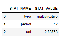
The result shows that a strong(with autocorrelation ~ 0.89) multiplicative yearly seasonality has been detected.
The corresponding decomposition result is illustrated as follows:
decomposed.collect()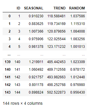
Values in the random components are all around 1, as expected.
In the following we apply the renowned variance test to the random component for anomaly detection(where the multiplier 3 is heuristically determined from the well-known 3?-rule for Gaussian random data, can be changed to other positive values).
from hana_ml.algorithms.pal.preprocessing import variance_test
test_res, _ = variance_test(data=decomposed,
                            key='ID',
                            data_col='RANDOM',
                            sigma_num=3)
In the anomaly detection result(i.e. the hana_ml.DataFrame test_res), anomalies are valued by 1 in its ‘IS_OUT_OF_RANGE’ column. Detailed info of the detected anomalies from the origin data can be obtained as follows:
anomalies_vt_id = cc.sql('SELECT ID FROM ({}) WHERE IS_OUT_OF_RANGE = 1'.format(test_res.select_statement))
anomalies_vt = cc.sql('SELECT * FROM ({}) WHERE ID IN ({})'.format(ap_df_wid.select_statement,
                                                                   anomalies_vt_id.select_statement))
anomalies_vt.collect()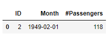
So a single anomaly with ID 2(corresponding to Febrary 1949) has been detected. However, there is some concern with this single anomaly point:
- firstly, the point is very close the starting time-limit, whose validity could be affected by extrapolations(required by the internal mechanism of the decomposition);
- secondly, the detected anomaly falls into the early stage of the time-series during which local level is still low, where multiplicative decomposition could be over-sensitive.
Another frequently used technique for anomaly detection is inter-quartile range(IQR) test, which is considered to be more robust to extreme anomalies. In the following we apply IQR test(with default multiplier, i.e. 1.5) to the random component of the decomposition result to see what should happen.
from hana_ml.algorithms.pal.stats import iqr
test_res, _ = iqr(data=decomposed, key='ID', col='RANDOM')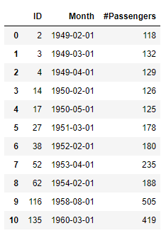
So, the anomaly point detected by variance test still remains in the IQR test result, along with the introduction of 10 newly detected anomalies. Let us inspect the corresponding residuals(i.e. random values) of these detected anomalies to determine how anomalous they are.
c.sql('SELECT * FROM ({}) WHERE ID IN (SELECT ID FROM ({}))'.format(decomposed[['ID', 'RANDOM']].select_statement, anomalies_iqr.select_statement)).collect()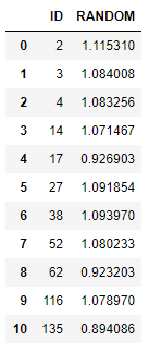
A noticeable newly detected anomaly is the one with ID 135(corresponding to March 1960), which deviates the most from 1 among all newly detected anomalies. Besides, it is in a time poistion where level values are high, and not that close to either time-limit of the given time-series as the point with ID 2.
Now let us visualize all detected anomalies in the random component under IQR test.
import matplotlib.pyplot as plt
import numpy as np
dc = decomposed.collect()
plt.plot(ap_data['Month'], dc['RANDOM'], 'k.-')
oidx = np.array(anomalies_iqr.collect()['ID']) - 1
plt.plot(ap_data['Month'][oidx], dc.iloc[oidx, 3], 'ro')
plt.show()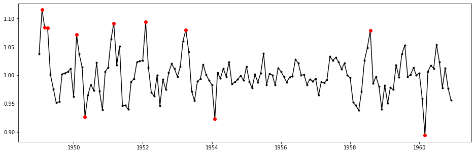
Detected anomalies can also be visulized from the original time-series, illustrated as follows:
import matplotlib.pyplot as plt
import numpy as np
ap_dc = ap_df.collect()
oidx = np.array(anomalies_iqr.collect()['ID']) - 1
plt.plot(ap_dc['Month'], ap_dc['#Passengers'], 'k.-')
plt.plot(ap_dc['Month'][oidx], ap_dc['#Passengers'][oidx], 'ro')
plt.show()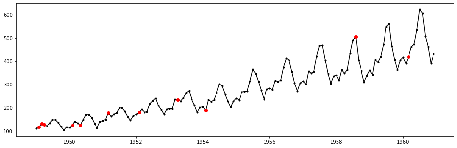
If knowing roughly how many anomalies are there in the dataset, then we can select only a specified number of data points with most deviant values(w.r.t. 1 for multiplicative seasonal decomposition) in the resiudual component. For example. if we expect that the number of anomalies in the dataset is 2, then can use the following line of code to select them out.
top2_anomalies = cc.sql('SELECT TOP 2 ID, RANDOM FROM ({}) ORDER BY ABS(RANDOM-1) DESC'.format(decomposed.select_statement))
top2_anomalies.collect()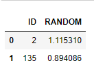
Visualization of the two points in the original dataset is also not difficult, with Python source code illustrated as follows:
import matplotlib.pyplot as plt
oidx = np.array(top2_anomalies.collect()['ID']) - 1
plt.plot(ap_dc['Month'], ap_dc['#Passengers'], 'k.-')
plt.plot(ap_dc['Month'][oidx], ap_dc['#Passengers'][oidx], 'ro')
plt.show()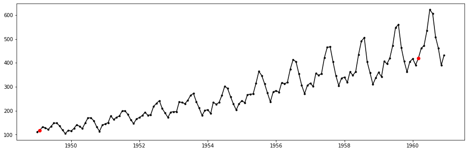
We see that the point with ID 135 still remains, and it is not likely to be a result of boundary extrapolation, so it may worth more investigation.
In the following section we try to decompose the AirPassenger dataset using additive seasonal decomposition model.
Additive Decomposition
As is known to all, a multiplicative model can be transformed to an additive one by taking logarithm transformation. So, if we apply logarithmic transform to the ‘#Passengers’ column in the dataset, then additive seasonal decomposition should be applicable to the transformed dataset, verified as follows:
ap_df_log = cc.sql('SELECT "ID", "Month", LN("#Passengers") FROM ({})'.format(ap_df_wid.select_statement))
stats_log, decomposed_log = seasonal_decompose(data = ap_df_log,
                                               key = 'ID',
                                               endog = 'LN(#Passengers)',
                                               extrapolation=True)
stats_log.collect()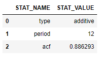
The seasonality test result shows that, after logarithmic transformation, a strong(with autocorrelation ~ 0.89) additive yearly seasonality has been detected in the transformed time-series.
Now let us check(the first 12 rows of) the decomposition result.
decomposed_log.head(12).collect()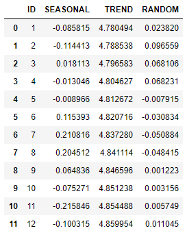
One can see that, different from multiplicative decomposition, values in the random component for additive decomposition are centered around 0, with reasons explained in the introduction section.
Again we apply 3?-rule of variance test to the RANDOM column in the decomposition result for detecting outliers.
test_res_log, _ = variance_test(data=decomposed_log, key='ID', data_col='RANDOM', sigma_num=3)
anomalies_log = cc.sql('SELECT ID, IS_OUT_OF_RANGE FROM ({}) WHERE IS_OUT_OF_RANGE = 1'.format(test_res.select_statement))
anomalies_log_pt = cc.sql('SELECT "ID", "Month", "LN(#Passengers)" FROM ({}) WHERE ID IN (SELECT ID FROM ({}))'.format(ap_df_log.select_statement, outliers.select_statement))
anomalies_log_pt.collect()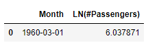
So a single anomaly has been detected, it can be visualized from the original time-series as follows:
import matplotlib.pyplot as plt
ap_dc= ap_df.collect()
plt.plot(ap_dc['Month'], ap_dc['#Passengers'], 'k.-')
tmsp = pd.to_datetime('1960-03-01')
plt.plot(tmsp, ap_dc[ap_dc['Month']==tmsp]['#Passengers'], 'ro')
plt.show()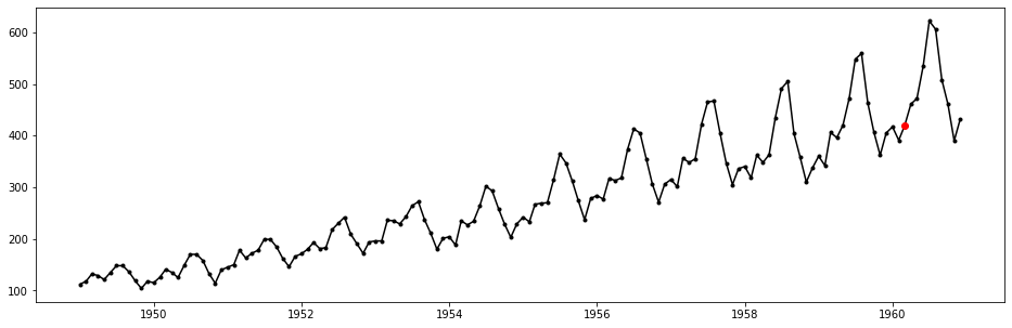
Red dot is the single anomaly point detected, which is also detected in the multiplicative decomposition model. This tells us that the number of airline passengers in March 1960 is highly likely to be anomalous.
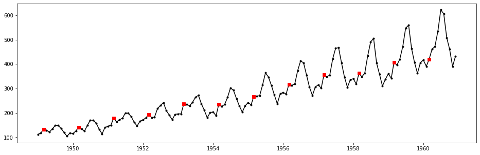
By inspecting data in previous years, we may find that the number of passengers will usually have a significant increment when moving from Febrary to March, followed by a slight drop down from March to April. However, in 1960 the proporition of increment from Febrary to March is only a little, while from March to April the increment becomes significant. This strongly voildates the regular seasonal pattern, and should be the reason why the point is labeled as anomalous. This can also be justified by the following plot, where the numbers of passengers in every March within the time-limits of the given time-series are marked by red squares.
Now let us try IQR test for anomaly detection.
test_res_log_iqr, _ = iqr(data=decomposed_log,
key='ID',
col='RANDOM')
anomalies_log_iqr_id = cc.sql('SELECT ID FROM ({}) WHERE IS_OUT_OF_RANGE = 1'.format(test_res_log_iqr.select_statement))
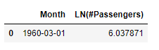
anomalies_log_iqr = cc.sql('SELECT "Month", "LN(#Passengers)" FROM ({}) WHERE ID IN ({})'.format(ap_df_log.select_statement,
anomalies_log_iqr_id.select_statement))
anomalies_log_iqr.collect()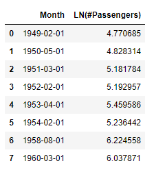
Again the data in March 1960 is labeled as anomalous. This time it is the most anomalous point in the sense that its residual value deviates the most from 0, verified as follows:
top1_anomaly_log_iqr_id = cc.sql('SELECT TOP 1 ID FROM ({}) ORDER BY ABS(RANDOM) DESC'.format(decomposed_log.select_statement))
top1_anomaly_log_iqr = cc.sql('SELECT "Month", "LN(#Passengers)" FROM ({}) WHERE ID IN ({})'.format(ap_df_log.select_statement, top1_anomaly_add_iqr_id.select_statement))
top1_anomaly_log_iqr.collect()