ABAP ADT Profiler(performance analysis)

Performance analysis has always been a challenge. Analysing the Performance trace result is even a bigger challenge.

SAP ABAP 7.5 Certification Preparation Guide

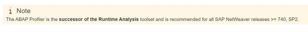
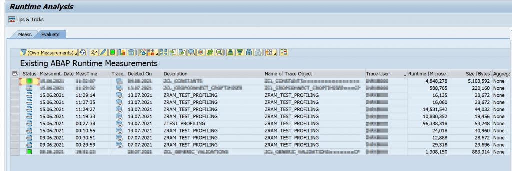
ABAP Profiler is the recommended tool going forward. Check the screenshot from the SAP itself.

ABAP Profiler is a powerful tool for analysing the runtime performance or to understand the flow of the code. But it can get really confusing with the different options to initiate the profiling, different tabs and columns to analyse the results.

1. Which option to choose?
   
2. What are the different tabs on the output?
   
3. What are all those columns and what do they mean?

Yes, all these details are available in our fav help.sap.com. Here is a simplified version of the same.

ABAP Profiler views

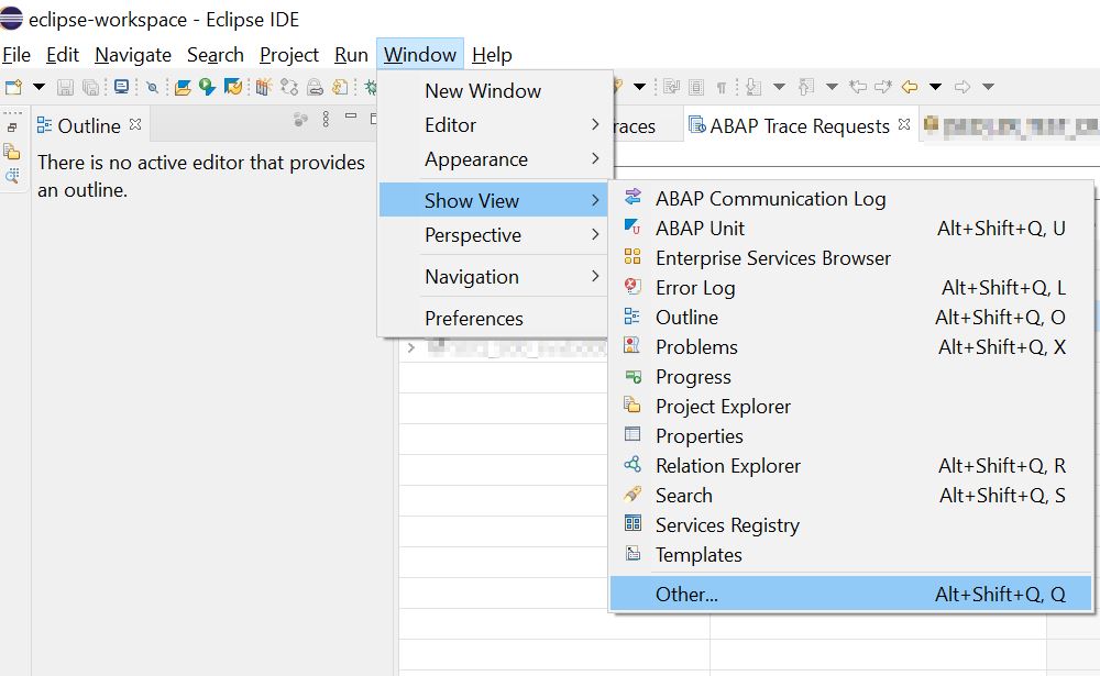
ADT has provided two views for working with ABAP Profiler.

1. ABAP Trace Requests to initiate the trace or view initiated trace requests.
   
2. ABAP Traces to view the trace results.

Initiate Profiling

Trace request can be initiated in one of the below three ways

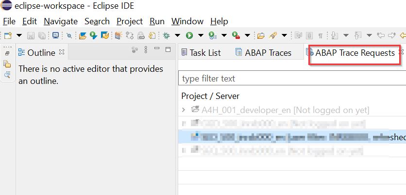
1. ABAP Trace Requests view

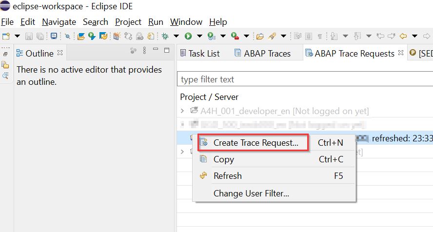
i. Open the ‘ABAP Trace Requests’ view.

ii. From the context menu of the project choose ‘Create Trace Request’

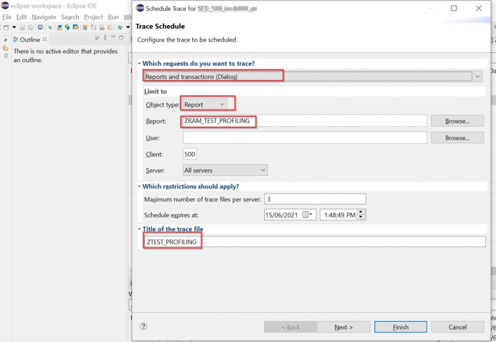
iii. Select the Type of Request, Object Type, Object Name, User (to restrict to a single user), ‘Title of the trace file’.

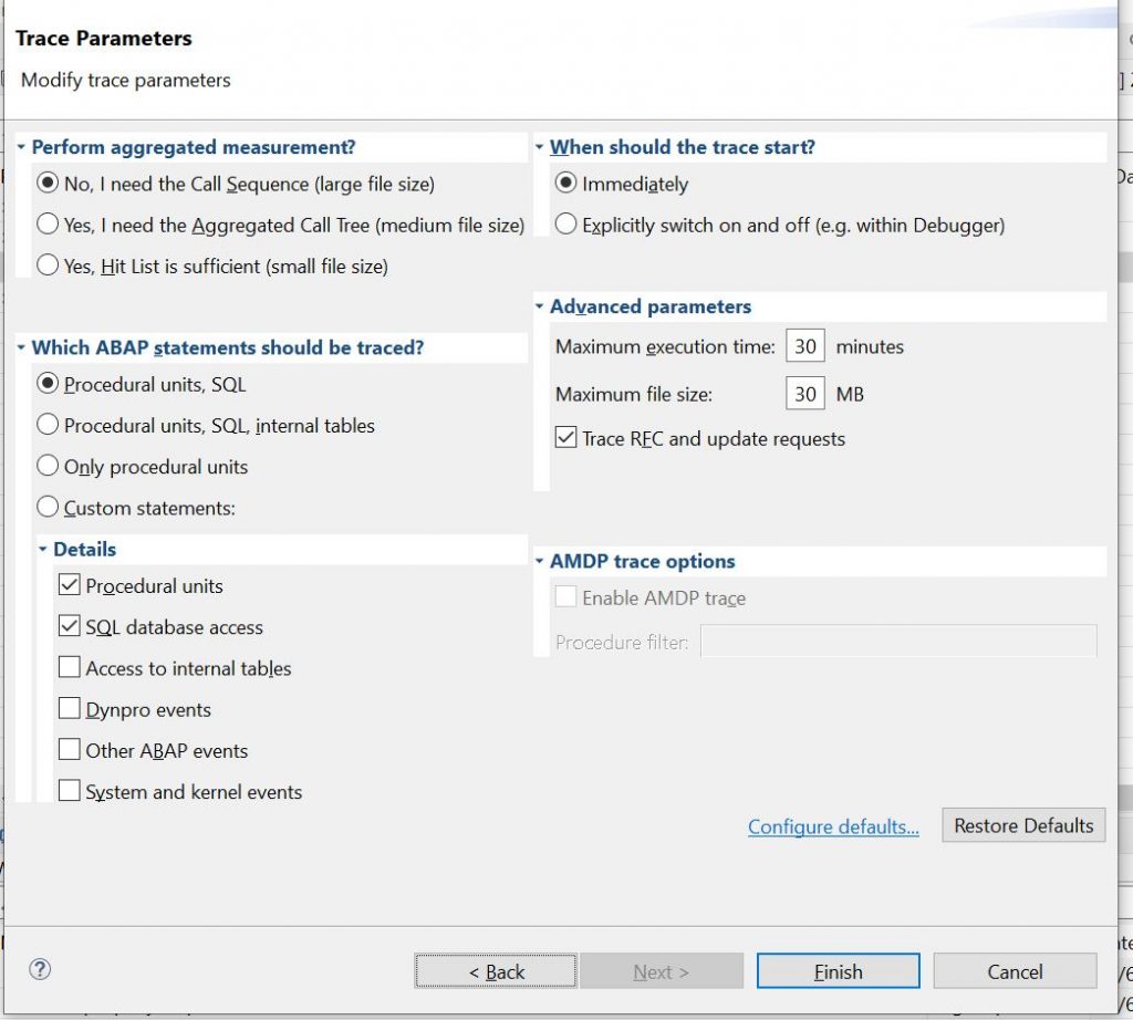
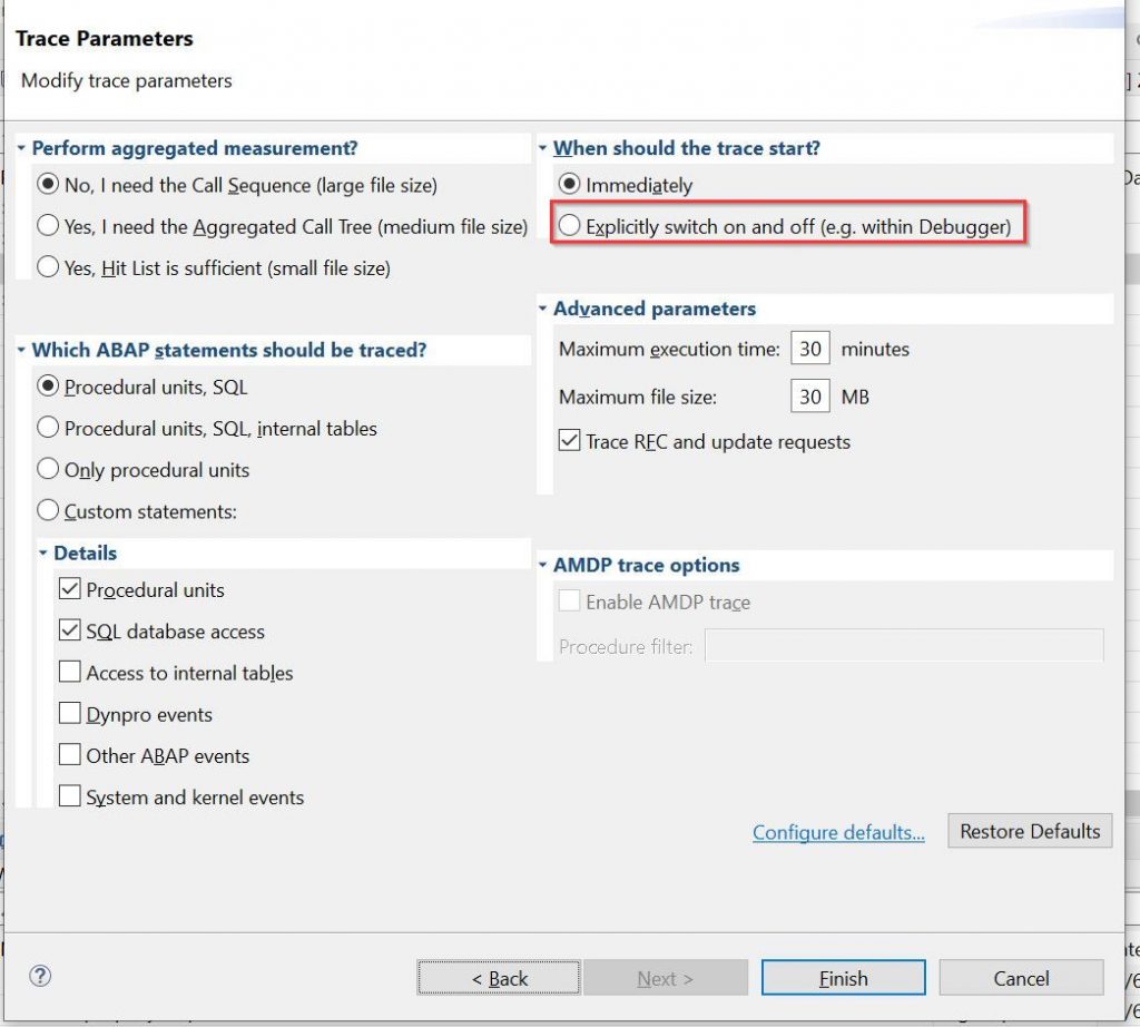
iv. On the next screen select the ‘Trace Parameters’ as required and click ‘Finish’.

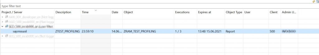
v. The newly created ‘Trace Request’ is visible on ‘ABAP Trace Requests’ view along with the number of executions as well.

2. ABAP Program

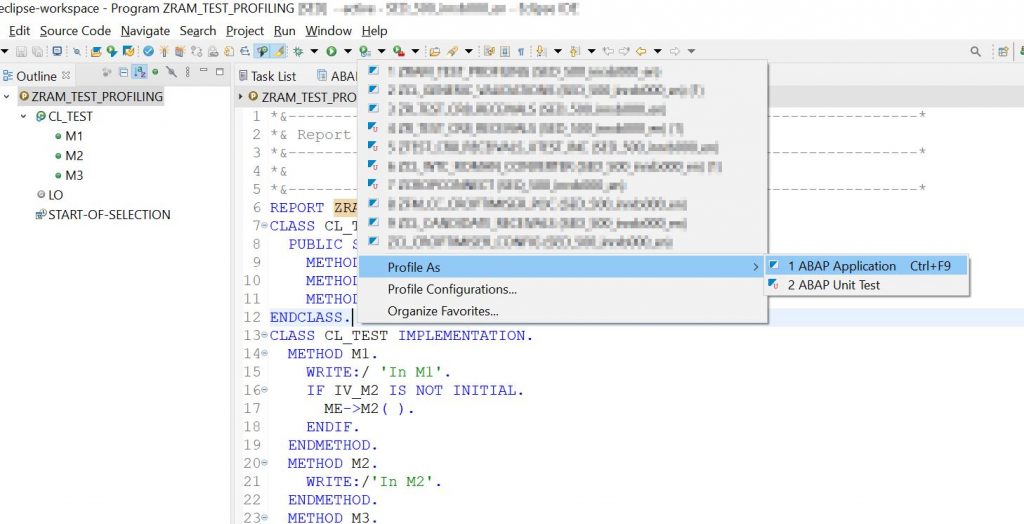
i. From the ABAP Program choose ‘Profile -> Profile As -> ABAP Application’ or Ctrl+F9. As you can see below profiling ‘ABAP Unit Test’ is also possible.

3. ABAP Debugger

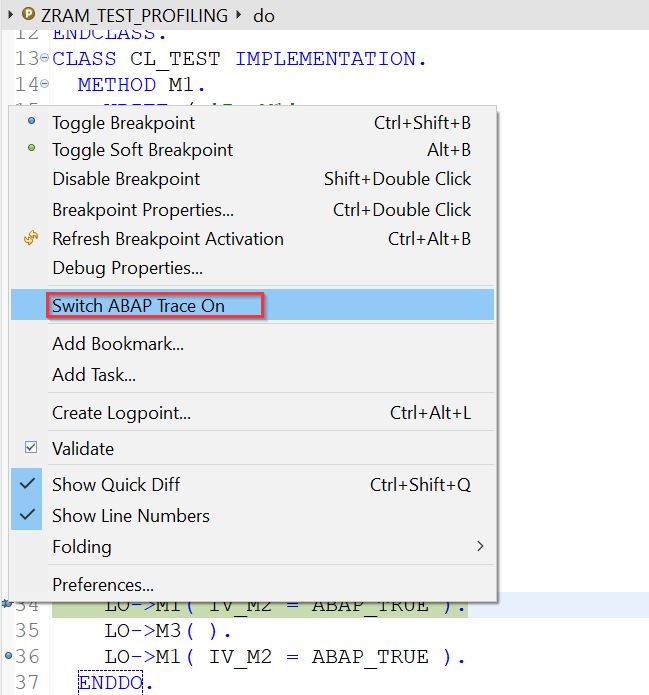
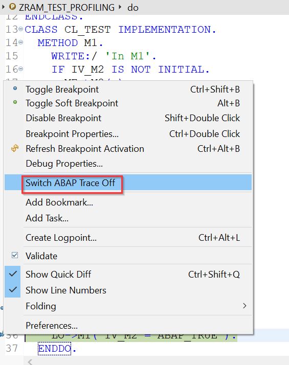
i. From ‘ABAP Trace Requests’ view create a request as before but select ‘Explicitly switch off and on’

ii. Now you can switch on and off the Profiler while debugging from the ruler context menu.

Trace Configurations

Once initiated the Profile configuration for the ABAP object is saved in ‘Profile->Profile Configurations’. These configurations can be edited as well. This helps in running the ABAP object with the same configuration next time via ‘Profile -> Profile As -> ABAP Application’ or Ctrl+F9.

SAT Transaction

All trace requests initiated from the ADT can be viewed in good old SAT transaction. But ABAP Profiling provides a more detailed view of the results when compared to SAT.

Terminology

Before we deep dive into the results let’s get familiar with the basic terminology.

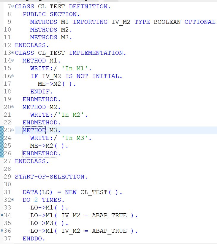
Let’s take the below ‘Example Analysis Program’ calling different methods of a class.

1. Call Position: Refers to the number of direct callers of a method and the call position of the calling method. A method can be called from many positions from the same calling method or program.

i. In the below example method M2 is called from 2 different call positions

1. ZRAM_TEST_PROFILING->M1->M2 at line 17
   
2. ZRAM_TEST_PROFILING->M3->M2 at line 25

ii. Method M1 is called from 3 positions

1. ZRAM_TEST_PROFILING->M1 at line 33
   
2. ZRAM_TEST_PROFILING->M1 at line 34
   
3. ZRAM_TEST_PROFILING->M1 at line 36

2. Call Stack: Is the list of names of methods called at run time from the beginning of a program until the execution of the current statement.

i. In the below example method M2 is called from 3 different call stacks

1. ZRAM_TEST_PROFILING->M1->M2 at line 34
   
2. ZRAM_TEST_PROFILING->M3->M2 at line 35
   
3. ZRAM_TEST_PROFILING->M1->M2 at line 36

3. Unspecified statements: Any intrinsic processing that the method is performing other than calling other methods or initiating objects for calling other methods or database access.

4. Specified statements: Any statements to initiate objects for calling other methods or select statements. Note that Specified statements does not include actual call to the other methods or the database access itself.

Example Analysis Program

Analyzing performance trace results

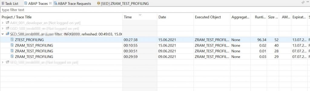
Captured traces can be viewed on the ‘ABAP Traces’ view.

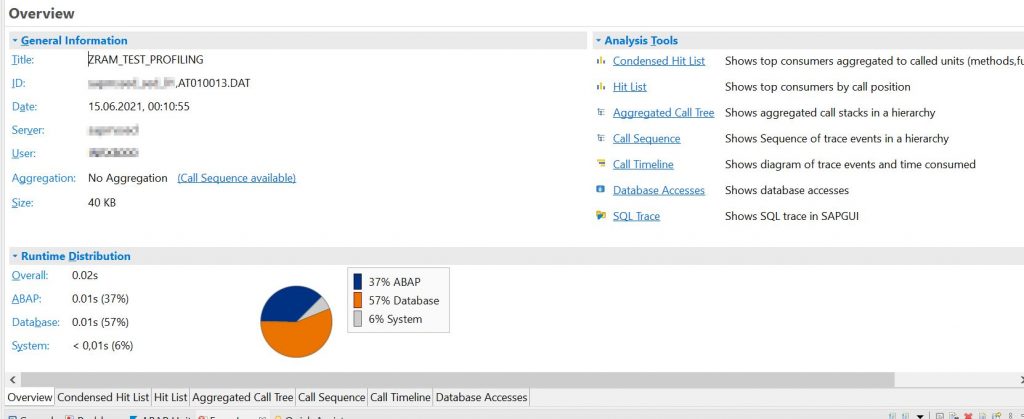
1. Overview screen

i. Open the Overview by double clicking the trace.
ii. Overview gives an Overall and percentage distribution of Runtime.

2. Condensed Hit List

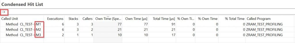
ii. Consolidated Hit List tab provides the unique called methods.

iii. Irrespective of the call position and call stack the called methods are specified only once in this tab.

iv. Let’s take the method M2 and describe the columns.

1. Example: M2 method is called from the below call stacks in a loop twice.

1. ZRAM_TEST_PROFILING->M1->M2 at line 34
   
2. ZRAM_TEST_PROFILING->M3->M2 at line 35
   
3. ZRAM_TEST_PROFILING->M1->M2 at line 36

v. Executions: specifies the number of times a given method is called irrespective of the call position and call stack.

1. Method M2 is executed 6 times irrespective of the call stacks.

vi. Stacks: specifies the number of different call stacks.

1. Method M2 is called from 3 different call stacks.

vii. Callers: specifies the number of callers irrespective of the call stack.

1. Method M2 is called by M1 and M3.

viii. Own Time(Specified and Unspecified in micro-seconds): Includes the time spent processing the intrinsic statements and statements to create objects to call other methods. Note that this does not include the time spent waiting for the other methods or select statements to finish.

1. In our example program there are no other objects or select statements. So, both this and ‘Own Time’ are same.

ix. Own Time(micro-seconds): Only the time taken by intrinsic statements of the method excluding any statements to create objects to call other methods.

x. Total Time(micro-seconds): Own Time + time taken by specified statements + time taken waiting for methods or select statements to finish.

1. Method M3 took 17 micro-seconds totally for the 2 iterations. Out of which it took only 10 micro-seconds for the intrinsic statements and 7 seconds for specified(if any) and waiting for M2 method to finish.

xi. %s: The above 3 fields are again specified in percentages.

3. Hit List

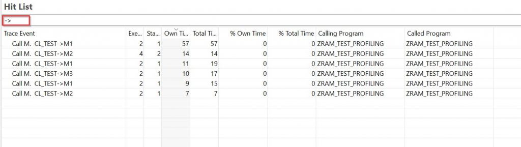
ii. Hit List tab provides the list of different call positions for each method.

1. M2 method is specified twice once on the second row and on the last row because of the 2 call positions from caller methods M1 and M3.

1. ZRAM_TEST_PROFILING->M1->M2 at line 17
   
2. ZRAM_TEST_PROFILING->M3->M2 at line 25

iii. As the Hit List is based on the call position, Callers column is not specified in this tab.

iv. There is no difference in the column list between Hit List and Consolidated Hit List other than Own Time(Specified and Unspecified in micro-seconds) and Callers columns missing.

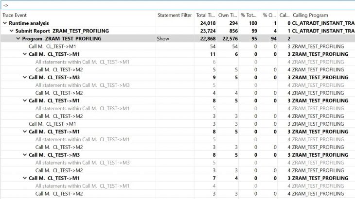
4. Aggregated Call Tree

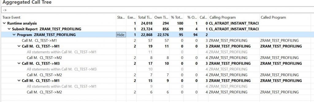
ii. Aggregated Call Tree tab provides the unique call stacks for each method.

iii. Let’s take the method M2 from the example program

1. Example: M2 method is called from the below call stacks in a loop twice.

1. ZRAM_TEST_PROFILING->M1->M2 at line 34
   
2. ZRAM_TEST_PROFILING->M3->M2 at line 35
   
3. ZRAM_TEST_PROFILING->M1->M2 at line 36

iv. Method M2 is called twice in each of the above call stacks totaling to 6 executions. But the Aggregated Call Tree specifies M2 only 3 times as it aggregated same call stack of M2 into a single call stack.

v. Most of the columns are same as Hit List.

5. Call Sequence

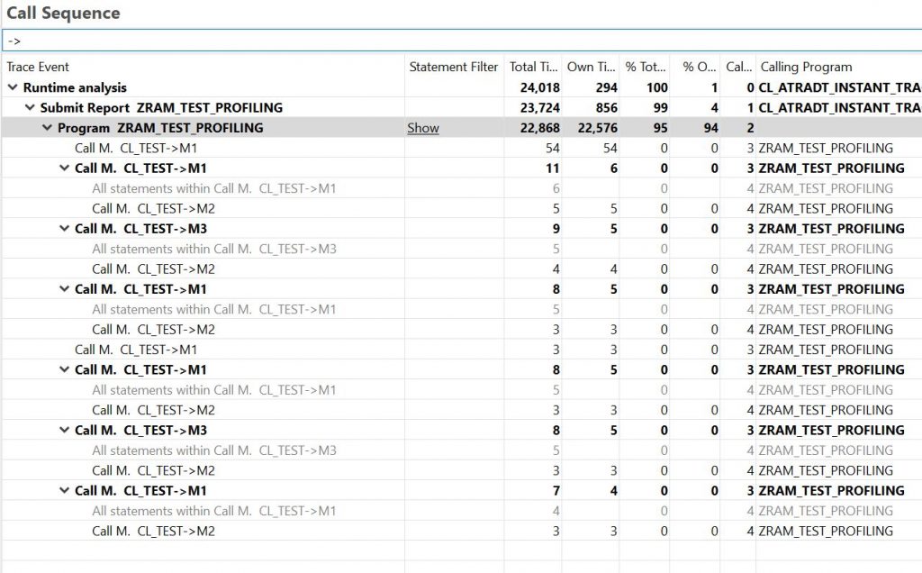
ii. Call Sequence tab provides the list of different call stacks and their sequence for each method.

iii. Let’s take the method M2 from the example program

1. Example: M2 method is called from the below call stacks in a loop twice.

1. ZRAM_TEST_PROFILING->M1->M2 at line 34
   
2. ZRAM_TEST_PROFILING->M3->M2 at line 35
   
3. ZRAM_TEST_PROFILING->M1->M2 at line 36

iv. Method M2 is called twice in each of the above call stacks totalling to 6 executions. So the Call sequence specified M2 6 times.

v. Most of the columns are same as Hit List.

6. Call Timeline

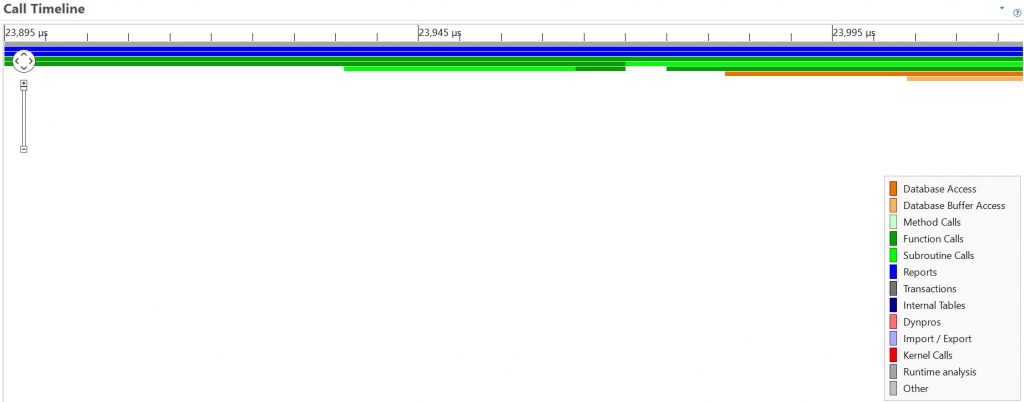
ii. Provides the graphical colour coded timeline of the runtime.

7. Database Accesses

i. Provides the SQL queries executed. In our example there are no SQL statements.

Tab summary

1. Hit List tab provides the list of different call positions for each method.
   
2. Consolidated Hit List tab provides the unique called methods.
   
3. Call Sequence tab provides the list of different call stacks and their sequence for each method.
   
4. Aggregated Call Tree tab provides the unique call stacks for each method.

Trace Parameters

With the basic understanding of different tabs on the results screen it is easy to understand the trace parameters. Let’s discuss some of the import options.

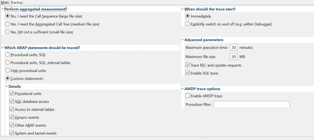
1. Perform aggregated measurement: Specifies the level of aggregation. Note that the file size increases as the level of detail increases.
   
2. Which ABAP statements should be trace: Only procedural or any specific custom events?
   
3. When should the trace start: We have already discussed this.